Example of a Neural Network Surrogate

Example of a Neural Network Surrogate#

Model for subcutaneous autoinjectors#

In this notebook, we’ll replicate Sree et. al. (2023) by creating a neural network (NN) surrogate of an expensive biomechanical model.

Background#

Autoinjectors are drug delivery devices that work kind of like an automated syringe. Basically, you put the device against the patient’s skin, press a button, and a spring within the device pushes the needle and drug is released into the patient.

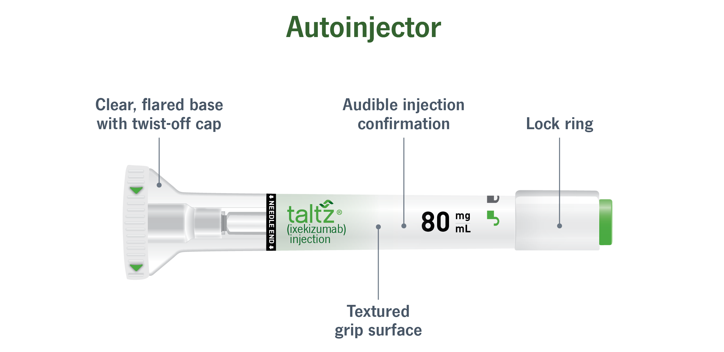
Picture of an autoinjector (taken from here).

To efficently design an optimal autoinjector, you need a computational model of the injection process. To this end, Sree et. al. (2023) present a biomechanical model for injections into subcutaneous tissue (i.e., the tissue right below your skin) via an autoinjector.

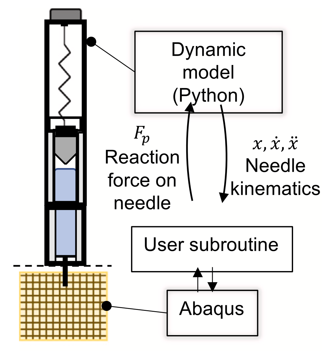
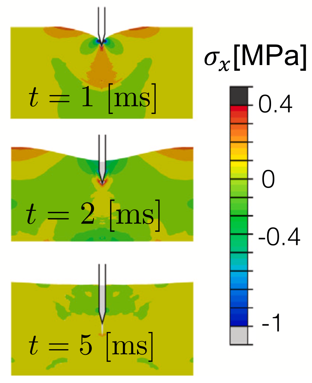
Left: Schematic of the autoinjector model. Right: Finite element simulation of tissue stress during injection. From Sree et. al. (2023).

The model, however, is expensive to evaluate—one evaluation takes multiple hours on several parallel processors. This is too slow for things like design optimization or uncertainty quantification. So we will speed it up by training a surrogate. Let’s get started.

Dataset#

To train the surrogate, we’ll use a dataset with thousands of evaluations of the expensive model (data was provided by the authors Sree et. al.). Let’s import the data:

The model has 10 inputs and 4 outputs. The inputs are things like drug viscosity, needle size, tissue biomechanical properties, etc. The outputs are the maximum acceleration/deceleration of fluid in syringe, the total time of injection, and the depth of needle insertion at the onset of drug delivery.

Preprocessing#

Ideally, we want the input and output data to be standarized and more-or-less evenly distributed. This helps avoid any numerical difficulties in training.

Let’s visualize the distribution of each input:

../../_images/b10beecbd48e4c2b3998701fbe81f8a26d47327aff0d6656062a68e8356c3c1d.svg

They are evenly distributed, but not standardized (i.e., the means and standard deviations are not 0 and 1, respectively). Let’s standardize the input data:

input_transform = StandardScaler(X_train.values)
X_train_scaled = vmap(input_transform.forward)(X_train.values)
X_test_scaled = vmap(input_transform.forward)(X_test.values)

Now let’s visualize the distribution of each output:

../../_images/d599a2bc625d30035a5a7fa074719980f252a745415adb237854a9bdca3aa4a6.svg

Some of the outputs are skewed. Let’s apply a log transformation, then standardize the output data:

def partial_log_transform(x):
    return jnp.hstack([x[0], jnp.log(x[1]), jnp.log(x[2]), x[3]])

def partial_exp_transform(y):
    return jnp.array([y[0], jnp.exp(y[1]), jnp.exp(y[2]), y[3]])

output_transform = StandardScaler(y_train.values, pretransform_forward=partial_log_transform, pretransform_inverse=partial_exp_transform)
y_train_scaled = vmap(output_transform.forward)(y_train.values)
y_test_scaled = vmap(output_transform.forward)(y_test.values)

Okay, now let’s visualize the transformed inputs and outputs:

../../_images/b93b3348f2c8e205203c61164b0b9fba62d1122e3765aecfac8f9b0ba60040e2.svg

../../_images/5cdd707753f442c866263a77203351731eaea08e78b5cc2bdfbc6754c8062a60.svg

Nice! The input/output data are all more-or-less evenly distributed and standardized. Now on to building the neural network surrogate.

Creating the NN surrogate#

Let’s set aside some of the training data for on-the-fly validation during training:

X_train_scaled_subset, X_val_scaled = jnp.split(X_train_scaled, [int(0.9 * X_train_scaled.shape[0])])
y_train_scaled_subset, y_val_scaled = jnp.split(y_train_scaled, [int(0.9 * y_train_scaled.shape[0])])

The best choice of neural network architecture is problem dependent. We’ll just use a simple MLP with 5 hidden layers and 100 neurons per layer.

Define the training loop:

Show code cell source Hide code cell source

def dataloader(X, y, batch_size, shuffle=True):
    num_samples = X.shape[0]
    indices = np.arange(num_samples)
    if shuffle:
        np.random.shuffle(indices)
    for start_idx in range(0, num_samples, batch_size):
        end_idx = min(start_idx + batch_size, num_samples)
        batch_indices = indices[start_idx:end_idx]
        yield X[batch_indices], y[batch_indices]

def train(
    batch_size: int,
    max_epochs: int,
    max_iters: int,
    learning_rate: float,
    X_train: Array,
    y_train: Array,
    X_val: Array,
    y_val: Array,
    loss_freq: int = 20,
    save_freq: int = 100,
    print_freq: int = 1000,
    *, 
    key
):
    if max_epochs is None and max_iters is None:
        raise ValueError("Either max_epochs or max_iters must be provided.")
    elif max_epochs is None:
        max_epochs = np.inf
    elif max_iters is None:
        max_iters = np.inf

    model = eqx.nn.MLP(in_size=10, out_size=4, width_size=100, depth=5, key=key)
    optimizer = optax.adam(learning_rate)
    optim_state = optimizer.init(eqx.filter(model, eqx.is_inexact_array))
    train_losses = []
    val_losses = []

    _epoch_counter, _iter_counter = 0, 0
    _reached_max_iters = False
    _accumulated_train_loss, _accumulated_val_loss, _N_loss = 0.0, 0.0, 0

    @eqx.filter_jit
    def compute_loss(model, X, y):
        y_pred = vmap(model)(X)
        return jnp.mean((y - y_pred)**2)

    @eqx.filter_jit
    def make_step(model, X, y, opt_state, optimizer):
        loss, grads = eqx.filter_value_and_grad(compute_loss)(model, X, y)
        updates, opt_state = optimizer.update(grads, opt_state)
        model = eqx.apply_updates(model, updates)
        return model, opt_state, loss
    
    # Training loop
    while _epoch_counter < max_epochs:
        for xb, yb in dataloader(X_train, y_train, batch_size):

            # Update the model
            model, optim_state, loss = make_step(model, xb, yb, optim_state, optimizer)
            
            # Add to the running loss totals
            if _iter_counter % loss_freq == 0:
                _accumulated_train_loss += loss
                _accumulated_val_loss += compute_loss(model, X_val, y_val)
                _N_loss += 1

            # Save the running average of the loss
            if _iter_counter % save_freq == 0:
                train_losses.append(_accumulated_train_loss/_N_loss)
                val_losses.append(_accumulated_val_loss/_N_loss)
                _accumulated_train_loss, _accumulated_val_loss, _N_loss = 0.0, 0.0, 0

            # Print the loss
            if _iter_counter % print_freq == 0:
                print(f"Epoch {_epoch_counter:<4}, iter {_iter_counter:<5}, train loss {train_losses[-1]:.4f}, val loss: {val_losses[-1]:.4f}")
            
            if _iter_counter >= max_iters:
                _reached_max_iters = True
                break
            _iter_counter += 1
        if _reached_max_iters:
            break
        _epoch_counter += 1

    return model, jnp.array(train_losses), jnp.array(val_losses)

Here is how to train the surrogate model using 500 points from the training set:

LOSS_FREQ, SAVE_FREQ, PRINT_FREQ = 20, 100, 1000
MAX_ITERS = 5000

key, subkey = jrandom.split(key)
trained_mlp, train_losses, val_losses = train(
    batch_size=128,
    max_epochs=None,
    max_iters=MAX_ITERS,
    learning_rate=1e-3,
    X_train=X_train_scaled_subset[:500],
    y_train=y_train_scaled_subset[:500],
    X_val=X_val_scaled,
    y_val=y_val_scaled,
    loss_freq=LOSS_FREQ,
    save_freq=SAVE_FREQ,
    print_freq=PRINT_FREQ,
    key=subkey
)

Epoch 0   , iter 0    , train loss 0.9686, val loss: 1.0007
Epoch 250 , iter 1000 , train loss 0.0012, val loss: 0.0219
Epoch 500 , iter 2000 , train loss 0.0002, val loss: 0.0212
Epoch 750 , iter 3000 , train loss 0.0003, val loss: 0.0205
Epoch 1000, iter 4000 , train loss 0.0001, val loss: 0.0201
Epoch 1250, iter 5000 , train loss 0.0003, val loss: 0.0199

../../_images/5a4dd34dadc8dca726c7ed0d145ce5b3c4828dd8115fbc536142997de5b05e70.svg

We now have a trained surrogate model.

Diagnostics: How good is the surrogate?#

The next question is: How accurate is our surrogate? We will use our test dataset to find out.

Parity plot#

Let’s plot the predicted output against the true output (for the test dataset), along with the root mean squared error (RMSE):

# Parity plot
y_train_pred = vmap(trained_mlp)(X_train_scaled)
y_test_pred = vmap(trained_mlp)(X_test_scaled)

# Root mean square error
rmse = lambda y, y_hat: jnp.sqrt(jnp.mean((y - y_hat)**2))

../../_images/986817c10c44186038ce410de0b6a9f7a56603c3ca0c5dbcf4e4a90d57768bfa.svg

../../_images/cba4093ab7bbe4276a29af1e5143caac499e395e759011985e45451b03c1cf23.svg

The closer the points are to the red line, the more accurate the surrogate is. This looks pretty good for only training on 500 points. Let’s try to improve it with more training data.

Convergence: How much data do we need?#

The more data you have available to train the surrogate, the better. In fact, you should see the prediction error go to zero as you increase the amount of training data (so long as the neural network is expressive enough and you train for long enough).

Let’s observe this convergence behavior by training the same neural network with different dataset sizes:

dataset_sizes = [100, 1000, 2500, 5000, 9000]
trained_mlps_N = {}
train_losses_N = {}
val_losses_N = {}

for N in dataset_sizes:
    print(f"Now training NN with dataset of size {N} ...\n")
    key, subkey = jrandom.split(key)
    trained_mlps_N[N], train_losses_N[N], val_losses_N[N] = train(
        batch_size=128,
        max_epochs=None,
        max_iters=MAX_ITERS,
        learning_rate=1e-3,
        X_train=X_train_scaled_subset[:N],
        y_train=y_train_scaled_subset[:N],
        X_val=X_val_scaled,
        y_val=y_val_scaled,
        loss_freq=LOSS_FREQ,
        save_freq=SAVE_FREQ,
        print_freq=PRINT_FREQ,
        key=subkey
    )
    print("\n...done.\n\n")

Now training NN with dataset of size 100 ...

Epoch 0   , iter 0    , train loss 1.0057, val loss: 1.0043
Epoch 1000, iter 1000 , train loss 0.0002, val loss: 0.0957
Epoch 2000, iter 2000 , train loss 0.0000, val loss: 0.0964
Epoch 3000, iter 3000 , train loss 0.0000, val loss: 0.0984
Epoch 4000, iter 4000 , train loss 0.0000, val loss: 0.0997
Epoch 5000, iter 5000 , train loss 0.0000, val loss: 0.1004

...done.


Now training NN with dataset of size 1000 ...

Epoch 0   , iter 0    , train loss 1.0383, val loss: 1.0080
Epoch 125 , iter 1000 , train loss 0.0029, val loss: 0.0142
Epoch 250 , iter 2000 , train loss 0.0010, val loss: 0.0119
Epoch 375 , iter 3000 , train loss 0.0008, val loss: 0.0118
Epoch 500 , iter 4000 , train loss 0.0006, val loss: 0.0116
Epoch 625 , iter 5000 , train loss 0.0004, val loss: 0.0115

...done.


Now training NN with dataset of size 2500 ...

Epoch 0   , iter 0    , train loss 1.0007, val loss: 1.0041
Epoch 50  , iter 1000 , train loss 0.0047, val loss: 0.0081
Epoch 100 , iter 2000 , train loss 0.0023, val loss: 0.0059
Epoch 150 , iter 3000 , train loss 0.0017, val loss: 0.0053
Epoch 200 , iter 4000 , train loss 0.0012, val loss: 0.0050
Epoch 250 , iter 5000 , train loss 0.0009, val loss: 0.0048

...done.


Now training NN with dataset of size 5000 ...

Epoch 0   , iter 0    , train loss 1.0061, val loss: 1.0060
Epoch 25  , iter 1000 , train loss 0.0057, val loss: 0.0079
Epoch 50  , iter 2000 , train loss 0.0038, val loss: 0.0054
Epoch 75  , iter 3000 , train loss 0.0032, val loss: 0.0050
Epoch 100 , iter 4000 , train loss 0.0020, val loss: 0.0040
Epoch 125 , iter 5000 , train loss 0.0016, val loss: 0.0037

...done.


Now training NN with dataset of size 9000 ...

Epoch 0   , iter 0    , train loss 1.0504, val loss: 1.0126
Epoch 14  , iter 1000 , train loss 0.0064, val loss: 0.0071
Epoch 28  , iter 2000 , train loss 0.0036, val loss: 0.0047
Epoch 42  , iter 3000 , train loss 0.0025, val loss: 0.0038
Epoch 56  , iter 4000 , train loss 0.0020, val loss: 0.0031
Epoch 70  , iter 5000 , train loss 0.0017, val loss: 0.0023

...done.

Let’s repeat the parity plots for different amounts of training data:

../../_images/f5f8b13933729d225b61d1c847c05f5bd1623655ae2ac5a9a8edc43d7e63ac7a.svg

../../_images/1e65a0018ab1360701f84333a52972840dea7102450afbdf1f0b72df9067fe17.svg

../../_images/3683d00c10145506efc8594597010fd2e0e968561f7b7205772fbff69d8260fa.svg

Again, the more data, the better. The fit for \(N=9,000\) is quite good.

Let’s plot the RMSE against the dataset size:

rmse_i = []
for N in dataset_sizes:
    y_test_pred = vmap(trained_mlps_N[N])(X_test_scaled)
    rmse_i.append(vmap(rmse, 1)(y_test_scaled, y_test_pred))
rmse_i = jnp.array(rmse_i)

../../_images/6bf0d0769d508840755e147de1bd040299d1624cd3c75922a5873e4c938aef52.svg

For this problem, the surrogate is pretty good when trained on 2,000 (or more) points. We could probably further improve accuracy by training for longer or using a different NN architecture.

Sensitivity analysis with surrogate#

Now that we have a trained and tested surrogate, there are many useful things we can do with it. As an example, we’ll demonstrate using the surrogate to do Sobol sensitivity analysis.

First, let’s create a helper function for evaluating the unscaled surrogate model.

def _surrogate(x, nn_model):
    x_scaled = input_transform.forward(x)
    y_scaled = nn_model(x_scaled)
    y = output_transform.inverse(y_scaled)
    return y

# This is the unscaled surrogate.
surrogate = partial(_surrogate, nn_model=trained_mlps_N[9000])

Now, let’s create bounds for the inputs (based on physical intuition and/or literature values):

import SALib.sample.sobol as sobol
import SALib.analyze.sobol as analyze_sobol

input_bounds_dict = {
    'viscosity_cP': [1.0, 20.0],
    'fill_volume_mL': [1.0, 1.05],
    'air_gap_height_mm': [4.0, 5.0],
    'needle_length_mm': [8.0, 15.9],
    'needle_diameter_mm': [0.133, 0.21],
    'spring_force_N': [18.0, 36.0],
    'spring_constant_N_per_mm': [150.0, 250.0],
    'kappa5': [0.0, 3.0],
    'kappa6': [0.0, 4.0],
    'kappa7': [0.0, 0.1]
}
input_bounds = np.array([[input_bounds_dict[i][0], input_bounds_dict[i][1]] for i in INPUT_NAMES])
print('The input bounds are:\n', input_bounds)

The input bounds are:
 [[1.00e+00 2.00e+01]
 [1.00e+00 1.05e+00]
 [4.00e+00 5.00e+00]
 [8.00e+00 1.59e+01]
 [1.33e-01 2.10e-01]
 [1.80e+01 3.60e+01]
 [1.50e+02 2.50e+02]
 [0.00e+00 3.00e+00]
 [0.00e+00 4.00e+00]
 [0.00e+00 1.00e-01]]

Next, we create Sobol samples of the inputs and pass them through the surrogate:

problem = {
    'num_vars': len(INPUT_NAMES),
    'names': INPUT_NAMES,
    'bounds': input_bounds
}

# The number of samples to generate (should be a power of 2).
N = 512

# Generate the samples.
sobol_samples = sobol.sample(problem, N, calc_second_order=False)

# Evaluate the surrogate model at the Sobol samples.
sobol_outputs = vmap(surrogate)(sobol_samples)

Finally, we calculate and plot the Sobol indices:

sobol_indices = {}
for i, o_name in enumerate(OUTPUT_NAMES):
    sobol_indices[o_name] = analyze_sobol.analyze(problem, sobol_outputs[:, i], calc_second_order=False, print_to_console=False)

../../_images/6822bad2e1bd3a1b1bd74ebe2a4582432c9fd57ccb412dcb89a4c9d43885b656.svg

Excellent! We now know to which inputs the outputs are most sensitive. For example, we can see that the injection time is very sensitive to the drug viscosity and needle diameter, somewhat sensitive to needle length and injector spring force, and not sensitive to any other inputs. This information can be used, for example, to further study and understand the physics behind the model, or to investigate how identifiable each parameter is given an experimental dataset.

Remember that sensitivity analysis would not have been feasible without a surrogate model—the true physical model was just too expensive. With a surrogate however, we can do sensitivity analysis, design optimization, uncertainty quantification, etc. all at a reasonable computational cost.