Second-Order Methods for Optimization

Second-Order Methods for Optimization#

Second order methods use the Hessians of the objective function to find the minimum. The Hessian is the matrix of second derivatives of the objective function. It is a symmetric matrix that contains information about the curvature of the function. Let \(f: \mathbb{R}^n \rightarrow \mathbb{R}\) be a twice differentiable function. The Hessian of \(f\) is the \(n \times n\) matrix of second partial derivatives of \(f\):

\[ \nabla^2 f(x) = \begin{bmatrix} \partial_i \partial_j f(x) \end{bmatrix}_{i,j=1}^n. \]

Another way to think about it is as the Jacobian of the gradient of \(f\):

\[ \nabla^2 f(x) = \nabla \left(\nabla f\right)(x). \]

Newton’s Method#

To motivate the method, start with a point \(x_t\) and suppose we want to move in the direction of a vector \(u\) (not necessarily a unit vector). We can approximate the function \(f\) by a second order Taylor expansion:

\[ f(x_t + u) \approx f(x_t) + \nabla f(x_t)^T u + \frac{1}{2} u^T \nabla^2 f(x_t) u. \]

What is the \(u\) that gives us the largest decrease in \(f\)? We need to minimize the right hand side of the above equation with respect to \(u\). The first order condition is:

\[ \nabla f(x_t) + \nabla^2 f(x_t) u = 0. \]

Assuming that \(\nabla^2 f(x_t)\) is invertible, we can solve for \(u\):

\[ u = - \left(\nabla^2 f(x_t)\right)^{-1} \nabla f(x_t). \]

The second condition is that the Hessian is positive definite. This ensures that the second order approximation is a convex function. If the Hessian is not positive definite, then the second order approximation may not be convex and the minimizer may not be a minimum. But so be it.

The Newton step is:

\[ x_{t+1} = x_t - \left(\nabla^2 f(x_t)\right)^{-1} \nabla f(x_t). \]

Typically, we move only \(\alpha \in (0,1]\) of the Newton step:

\[ x_{t+1} = x_t - \alpha \left(\nabla^2 f(x_t)\right)^{-1} \nabla f(x_t). \]

Unfortunately, it is not implemented in optax. But we can implement it ourselves.

from jax import value_and_grad, hessian
import jax.numpy as jnp
import equinox as eqx


def newton_raphson(f, x0, args=(), alpha=0.1, n_iter=10, return_path=False):
    pf = value_and_grad(f)
    p2f = hessian(f)
    
    @eqx.filter_jit
    def step(x, args):
        l, g = pf(x, *args)
        g2 = p2f(x, *args)
        
        # Technical things to make it work with pytrees
        g = jnp.stack(jax.tree_util.tree_leaves(g), axis=0)
        g2 = jnp.stack(jax.tree_util.tree_leaves(g2), axis=0)
        # end of technical stuff

        # Solve the linear system
        u = jnp.linalg.solve(g2, g[..., None])[..., 0]

        # Pytree stuff again
        u = jax.tree_util.tree_unflatten(jax.tree_util.tree_structure(x), u)
        # end of pytree stuff

        # Update (but for pytrees)
        new_x = jax.tree_util.tree_map(lambda xi, ui: xi - alpha * ui, x, u)

        return l, new_x
    
    x = x0
    path = [x0]
    fs = []
    for i in range(n_iter):
        l, x = step(x, args)
        path.append(x)
        fs.append(l)
    if return_path:
        return x, path, fs
    return x

Generate our previous dataset and the model:

import jax.random as jrandom

key = jrandom.PRNGKey(0)

# Generate some synthetic data
N = 1_000
X = jrandom.normal(key, (N,))
key, subkey = jrandom.split(key)
y = 1.5 * X ** 2 - 2 * X + jrandom.normal(subkey, (N,)) * 0.5

# Make also a test set (here an ideal one)
N_test = 50
X_test = jnp.linspace(-3, 3, N_test)
key, subkey = jrandom.split(key)
y_test = 1.5 * X_test ** 2 - 2 * X_test + jrandom.normal(subkey, (N_test,)) * 0.5

import numpy as np
import equinox as eqx
import jax
from functools import partial


class MyModel(eqx.Module):
    theta: jax.Array

    def __init__(self, key):
        self.theta = jax.random.normal(key, (3,))
    
    @partial(jax.vmap, in_axes=(None, 0))
    def __call__(self, x):
        return self.theta @ jnp.array([1, x, x ** 2])

Here is how to use the algorithm:

key, subkey = jrandom.split(key)

# The model
model = MyModel(subkey)

# The loss
@eqx.filter_jit
def loss(model, x, y):
    return jnp.mean((model(x) - y) ** 2)

model, path, losses = newton_raphson(
    loss,
    model,
    args=(X, y),
    alpha=0.5,
    n_iter=10,
    return_path=True
)

Here is how it performs in our simple example:

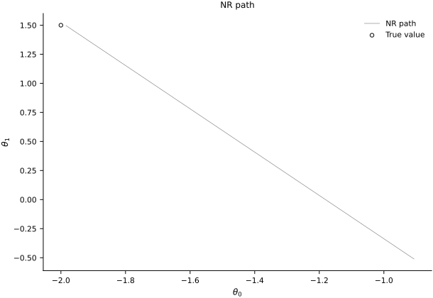
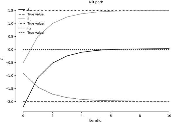
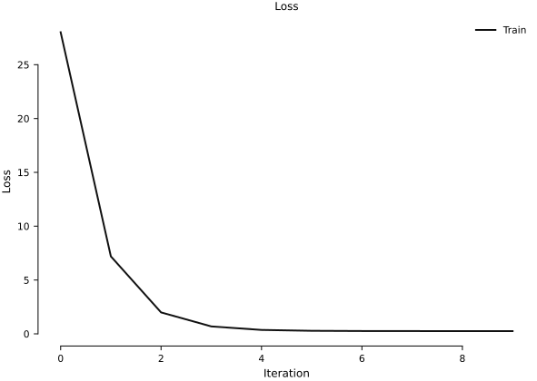
Three Newton-method diagnostics: the coefficient-plane path, coefficient traces against generating values, and the rapidly decreasing training loss.

I hope that you can see that the algorithm is super fast. As a matter of fact, in this particular example it converges in one iteration if you set the learning rate to 1. Why?

There is a catch though. The algorithm requires second derivatives of the objective function. In practice, it is not always possible to compute them. In addition, the Hessian matrix is \(n \times n\) and it is not always possible to invert it. Matrix inversion is computationally expensive: inverting an \(n \times n\) dense matrix costs \(O(n^3)\). This is not going to work for large \(n\) unless the Hessian is sparse, which is generally not the case when training neural networks.

Broyden-Fletcher-Goldfarb-Shanno (BFGS) Method#

The BFGS method is a quasi-Newton method. It uses an approximation of the Hessian matrix and updates that approximation at each iteration. The algorithm is as follows:

Initialize \(x_0\) and \(H_0\).
For \(t=0,1,2,\ldots\):
1. Compute the search direction \(d_t = -H_t^{-1} \nabla f(x_t)\).
2. Line search: find \(\alpha_t\) such that \(f(x_t + \alpha_t d_t) = \min_{\alpha \geq 0} f(x_t + \alpha d_t)\).
3. Update \(x_{t+1} = x_t + \alpha_t d_t\).
4. Update \(H_{t+1}\).

The BFGS update and its convergence properties are developed by Nocedal and Wright (2006).

This is also not a good algorithm for training neural networks. This is because the matrix \(H_t\) is also \(n \times n\). So, this is not a good algorithm for large \(n\).

Limited-memory BFGS (L-BFGS) Method#

This version of the BFGS method does not store \(n \times n\) matrices. It constructs each search direction from a limited history of parameter and gradient differences (Nocedal and Wright, 2006). This is a good algorithm for training models in many cases. When should you use it?

When you have a relatively small dataset so that each evaluation of the objective function is not too expensive. This is because the algorithm requires processing all the data at each iteration.
When a local optimization method is appropriate. For a general nonconvex problem, the outcome depends on initialization and is not guaranteed to be a minimum.
Multiple runs from different initializations can help compare candidate solutions.

Both Optax and JAXopt provide L-BFGS. We use JAXopt here. Let’s play with it.

import jaxopt

model = MyModel(subkey)

opt = jaxopt.LBFGS(loss, maxiter=10, jit=True)

n_iter = 20

opt_state = opt.init_state(model, X, y)

path = [model]
losses = [opt_state.value]

for i in range(n_iter):
    model, opt_state = opt.update(model, opt_state, X, y)
    path.append(model)
    losses.append(opt_state.value)

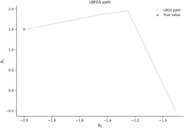
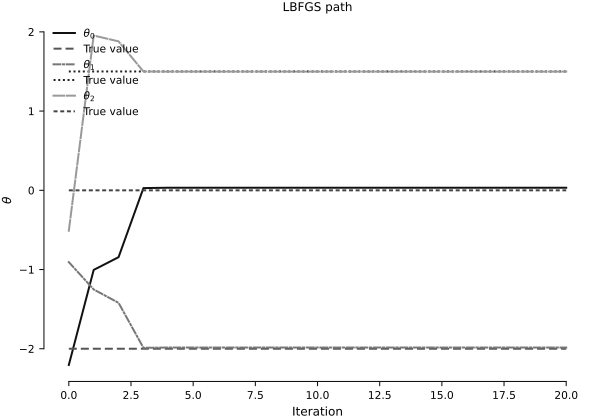
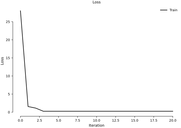
Here are the results:

Three limited-memory BFGS diagnostics: the coefficient-plane path, coefficient traces against generating values, and the decreasing training loss.

Stochastic second-order methods#

There are some stochastic second-order methods that can process the data in minibatches, but they are not commonly used. A multi-batch L-BFGS method is developed by Berahas et al. (2016).