Show code cell source

Hide code cell source

import matplotlib.pyplot as plt
%matplotlib inline
import matplotlib_inline
matplotlib_inline.backend_inline.set_matplotlib_formats('svg', 'pdf')
import seaborn as sns

import equinox
import optax

Show code cell source

Hide code cell source

import jax
import equinox as eqx

class FourierEncoding(eqx.Module):
    B: jax.Array

    @property
    def num_fourier_features(self) -> int:
        return self.B.shape[0]

    @property
    def in_size(self) -> int:
        return self.B.shape[1]
    
    @property
    def out_size(self) -> int:
        return self.B.shape[0] * 2

    def __init__(self, 
                 in_size: int, 
                 num_fourier_features: int, 
                 key: jax.random.PRNGKey, 
                 sigma: float = 1.0):
        self.B = jax.random.normal(
            key, shape=(num_fourier_features, in_size),
            dtype=jax.numpy.float32) * sigma
    
    def __call__(self, x: jax.Array, **kwargs) -> jax.Array:
        return jax.numpy.concatenate(
            [jax.numpy.cos(jax.numpy.dot(self.B, x)),
             jax.numpy.sin(jax.numpy.dot(self.B, x))],
            axis=0)
    

def train_pinn(
        loss,
        fourier_mlp,
        key,
        optimizer,
        filter_spec,
        Lx=1.0,
        Ly=1.0,
        num_collocation_residual=512,
        num_iter=10_000,
        freq=1,
    ):

    # this is new
    def new_loss(diff_model, static_model, x, y):
        comb_model = eqx.combine(diff_model, static_model)
        return loss(comb_model, x, y)

    @eqx.filter_jit
    def step(opt_state, model, xs, ys):
        # added this line
        diff_model, static_model = eqx.partition(model, filter_spec)
        # changed the loss to the new loss
        value, grads = eqx.filter_value_and_grad(new_loss)(diff_model, static_model, xs, ys)
        updates, opt_state = optimizer.update(grads, opt_state)
        model = eqx.apply_updates(model, updates)
        return model, opt_state, value
    
    opt_state = optimizer.init(eqx.filter(fourier_mlp, eqx.is_inexact_array))
    
    losses = []
    for i in range(num_iter):
        key1, key2, key = jrandom.split(key, 3)
        xb = jrandom.uniform(key1, (num_collocation_residual,), maxval=Lx)
        yb = jrandom.uniform(key2, (num_collocation_residual,), maxval=Ly)
        fourier_mlp, opt_state, value = step(opt_state, fourier_mlp, xb, yb)
        if i % freq == 0:
            losses.append(value)
            print(f"Step {i}, residual loss {value:.3e}")
    return fourier_mlp, losses

Energy Functionals

Consider the steady-state heat equation on the rectangle \(\Omega=[0,L_x]\times[0,L_y]\), with constant conductivity \(k>0\), a continuous source \(f\), and zero boundary temperature:

\[\begin{split} \begin{aligned} -k\Delta u &= f &&\text{in }\Omega,\\ u &=0 &&\text{on }\partial\Omega. \end{aligned} \end{split}\]

The integrated squared residual assigns a scalar to each candidate field:

\[ R[u]=\int_\Omega(-k\Delta u-f)^2\,dx\,dy. \]

A map from a function to a scalar is called a functional. For this equation, the energy functional is

\[ E[u]=\int_\Omega\left(\frac{k}{2}|\nabla u|^2-fu\right)\,dx\,dy. \]

Unlike the squared residual, this energy uses only first derivatives. Its admissible fields have square-integrable values and first weak derivatives and satisfy the zero boundary condition. A weak derivative extends differentiation through integration against smooth test functions; it allows fields with corners, such as ReLU-network outputs. This admissible space is denoted \(W_0^{1,2}(\Omega)\); the subscript records the zero boundary values (Adams and Fournier, 2003).

Under the assumptions above, the energy has a unique minimizer in this space. The minimizer is a weak solution: it satisfies an integrated form of the heat equation, even when classical second derivatives are unavailable. A sufficiently smooth weak solution also satisfies the PDE pointwise. Restricting the candidates to a neural-network family does not guarantee a unique set of weights or successful optimization.

Let \(v\in W_0^{1,2}(\Omega)\) be a perturbation that preserves the boundary values. The first variation measures the change in energy in direction \(v\):

\[ \frac{\delta E[u]}{\delta v} =\left.\frac{d}{d\epsilon}E[u+\epsilon v]\right|_{\epsilon=0} =\int_\Omega(k\nabla u\cdot\nabla v-fv)\,dx\,dy. \]

At a minimizer this expression is zero for every admissible \(v\). That integrated identity is the weak heat equation; it only requires first derivatives of \(u\).

If \(u\) is sufficiently smooth, integration by parts gives

\[ \int_\Omega(k\nabla u\cdot\nabla v-fv)\,dx\,dy =\int_\Omega(-k\Delta u-f)v\,dx\,dy. \]

The boundary term vanishes because \(v=0\) there. Since the identity holds for every test function, the smooth field satisfies the heat equation. This calculation interprets the weak equation in the smooth case; it does not assume that every admissible field has a classical Laplacian.

The second variation is \(k\int_\Omega|\nabla v|^2\,dx\,dy\). Positive conductivity and the fixed zero boundary values make the energy strictly convex in the field, which explains uniqueness of its minimizer.

Nondimensionalizing the Energy Functional

We scale everything like we did before:

\begin{align*} x &\mapsto \tilde{x} = \frac{x}{L_x}, \ y &\mapsto \tilde{y} = \frac{y}{L_y}, \ u &\mapsto \tilde{u} = \frac{u}{u_s}, \ f &\mapsto \tilde{f} = \frac{f}{f_s}. \ \end{align*}

We can now directly make the change on the energy functional:

\begin{align*} E[u] &= L_xL_y\int_{\tilde{\Omega}} \left{ \frac{1}{2}\left[\frac{ku_s^2}{L_x^2}\left(\frac{\partial \tilde{u}}{\partial \tilde{x}}\right)^2 + \frac{ku_s^2}{L_y^2}\left(\frac{\partial \tilde{u}}{\partial \tilde{y}}\right)^2\right] - f_su_s\tilde{f}\tilde{u} \right} , d\tilde{x} , d\tilde{y} \ &= L_xL_yf_su_s \int_{\tilde{\Omega}} \left{ \frac{1}{2}\left[\frac{ku_s}{L_x^2f_s}\left(\frac{\partial \tilde{u}}{\partial \tilde{x}}\right)^2 + \frac{ku_s}{L_y^2f_s}\left(\frac{\partial \tilde{u}}{\partial \tilde{y}}\right)^2\right] - \tilde{f}\tilde{u} \right} , d\tilde{x} , d\tilde{y} \ &= L_xL_yf_su_s \int_{\tilde{\Omega}} \left{ \frac{1}{2}\left[k_x\left(\frac{\partial \tilde{u}}{\partial \tilde{x}}\right)^2 + k_y\left(\frac{\partial \tilde{u}}{\partial \tilde{y}}\right)^2\right] - \tilde{f}\tilde{u} \right} , d\tilde{x} , d\tilde{y}, \ &= L_xL_yf_su_s \tilde{E}[\tilde{u}], \end{align*}

where we have defined \(k_x = \frac{ku_s}{L_x^2f_s}\) and \(k_y = \frac{ku_s}{L_y^2f_s}\).

We will pick \(u_s\) to make the two terms inside \(\tilde{E}[\tilde{u}]\) have the same order of magnitude. So, we pick:

\begin{align*} &\left|k_x\left(\frac{\partial \tilde{u}}{\partial \tilde{x}}\right)^2+ k_y\left(\frac{\partial \tilde{u}}{\partial \tilde{y}}\right)^2\right|{\infty} = |\tilde{f}\tilde{u}|{\infty}, \ &\implies \frac{ku_s}{f_s} \left|L_x^{-2}\left(\frac{\partial \tilde{u}}{\partial \tilde{x}}\right)^2+ L_y^{-2}\left(\frac{\partial \tilde{u}}{\partial \tilde{y}}\right)^2\right|{\infty} = |\tilde{f}\tilde{u}|{\infty}, \ &\implies u_s = \frac{f_s}{k}|\tilde{f}\tilde{u}|{\infty}\left|L_x^{-2}\left(\frac{\partial \tilde{u}}{\partial \tilde{x}}\right)^2+ L_y^{-2}\left(\frac{\partial \tilde{u}}{\partial \tilde{y}}\right)^2\right|{\infty}^{-1}. \end{align*}

At the same time, we want to make both terms to be of order one. This can be achieved by picking:

\[ \|\tilde{f}\tilde{u}\|_{\infty} = 1. \]

or

\[ f_s = \|f(\tilde{x}L_x, \tilde{y}L_y)\tilde{u}\|_{\infty}. \]

We evaluate the norms using the randomly initialized network and then hold the scales fixed during training. This is an initialization-dependent balancing heuristic, not a uniquely determined physical choice of units.

Start with our problem definition:

import jax.numpy as jnp

u0 = 500 # degrees Kelvin
k = 10.0 # thermal conductivity in W/mK
Lx = 0.1 # meters
Ly = 1.0 # meters

f = lambda x, y: 2.0 * jnp.pi ** 2 * k * u0 * (
    -Lx ** 2 * jnp.sin(jnp.pi * x / Lx) ** 2 * jnp.cos(2.0 * jnp.pi * y / Ly)
    -Ly ** 2 * jnp.sin(jnp.pi * y / Ly) ** 2 * jnp.cos(2.0 * jnp.pi * x / Lx)
) / (Lx ** 2 * Ly ** 2)

Some of the scaling:

to_x = lambda xt: xt * Lx
to_y = lambda yt: yt * Ly
to_xt = lambda x: x / Lx
to_yt = lambda y: y / Ly

For \(u_s\), we need to parameterize the field:

# Make our model
import jax
import jax.random as jrandom
key = jrandom.PRNGKey(0)

key1, key2, key = jrandom.split(key, 3)
num_fourier_features = 100
width = 256
depth = 4
model = eqx.nn.Sequential([
    FourierEncoding(2, num_fourier_features, key1),
    eqx.nn.MLP(2 * num_fourier_features, 'scalar', width, depth, jax.nn.tanh, key=key2),
])
ut = lambda xt, yt, model: xt * (1 - xt) * yt * (1 - yt) * model(jnp.array([xt, yt]))

Some code to calculate infinity norms of functions using points:

jit_vmap = lambda g: jit(vmap(g, in_axes=(0, 0)))
infinity_norm = lambda g, xs, ys: jnp.max(jnp.abs(jit_vmap(g)(xs, ys)))

Now, we can find \(f_s\):

from jax import vmap, jit

xs = jnp.linspace(0, Lx, 100)
ys = jnp.linspace(0, Ly, 100)
X, Y = jnp.meshgrid(xs, ys)
Xt = to_xt(X)
Yt = to_yt(Y)
Xt_flat = Xt.flatten()
Yt_flat = Yt.flatten()

fs = infinity_norm(lambda xt, yt: f(to_x(xt), to_y(yt)) * ut(xt, yt, model), Xt_flat, Yt_flat)

# The scaled version of the source
ft = lambda xt, yt: f(to_x(xt), to_y(yt)) / fs

print(f"fs = {fs:.3e}")

fs = 2.016e+04

And we can find \(u_s\):

term1 = jit(vmap(lambda xt, yt: jnp.abs(ft(xt, yt) * ut(xt, yt, model)), in_axes=(0, 0)))(Xt_flat, Yt_flat).max()

from jax import grad
ut_x = grad(ut, 0)
ut_y = grad(ut, 1)
term2 = infinity_norm(lambda xt, yt: ut_x(xt, yt, model) ** 2 / Lx ** 2 + ut_y(xt, yt, model) **2 / Ly ** 2, Xt_flat, Yt_flat)

us = (fs * term1) / (k * term2)

print(f"us = {us:.3e}")

us = 6.231e+04

Now, we can define the scaled energy thermal conductivity:

kx = (k * us) / (Lx ** 2  * fs)
ky = (k * us) / (Ly ** 2  * fs)

print(f"kx = {kx:.3e}, ky = {ky:.3e}")

kx = 3.091e+03, ky = 3.091e+01

The following diagnostic uses the same x- and y-gradient coefficients as the training loss.

tE_term1 = jit(vmap(lambda xt, yt: 0.5 * (kx * ut_x(xt, yt, model) ** 2 + ky * ut_y(xt, yt, model) ** 2), in_axes=(0, 0)))
tE_term2 = jit(vmap(lambda xt, yt: ft(xt, yt) * ut(xt, yt, model), in_axes=(0, 0)))


fig, ax = plt.subplots(1,2, figsize=FIGURE_SIZES["full_landscape"])
trm1 = tE_term1(Xt_flat, Yt_flat).reshape(X.shape)
c = ax[0].contourf(Xt, Yt, trm1, cmap='viridis')
fig.colorbar(c, ax=ax[0])
ax[0].set_xlabel(r'$\tilde{x}$')
ax[0].set_ylabel(r'$\tilde{y}$')

trm2 = tE_term2(Xt_flat, Yt_flat).reshape(X.shape)
c = ax[1].contourf(Xt, Yt, trm2, cmap='viridis')
fig.colorbar(c, ax=ax[1])
ax[1].set_xlabel(r'$\tilde{x}$')
ax[1].set_ylabel(r'$\tilde{y}$')

finalize_axes(keep_box=True)
plt.tight_layout();

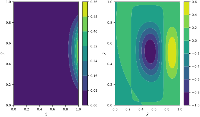
The two terms now have comparable scales at initialization. Training can change that balance.

Training the Network

Let’s make our new loss:

energy_loss = vmap(
    lambda xt, yt, model: 0.5 * (kx * ut_x(xt, yt, model) ** 2 + ky * ut_y(xt, yt, model) ** 2) - ft(xt, yt) * ut(xt, yt, model),
    in_axes=(0, 0, None),
)
pinn_loss = lambda model, xt, yt: jnp.mean(energy_loss(xt, yt, model))

import optax
import jax.tree_util as jtu

# Here, I am actually optimizing the Fourier coefficients
filter_spec = jtu.tree_map(lambda _: True, model)

key, subkey = jax.random.split(key)
optimizer = optax.adam(1e-3)
trained_model, losses = train_pinn(
    pinn_loss, model, subkey, optimizer, filter_spec,
    num_collocation_residual=256, num_iter=5_000, freq=100, Lx=1.0, Ly=1.0)

Step 0, residual loss 1.109e-01

Step 100, residual loss -8.265e-02

Step 200, residual loss -1.764e-01

Step 300, residual loss -2.119e-01

Step 400, residual loss -1.290e-01

Step 500, residual loss -1.986e-01

Step 600, residual loss -2.048e-01

Step 700, residual loss -2.150e-01

Step 800, residual loss -1.771e-01

Step 900, residual loss -1.811e-01

Step 1000, residual loss -1.491e-01

Step 1100, residual loss -9.115e-02

Step 1200, residual loss -1.801e-01

Step 1300, residual loss -1.807e-01

Step 1400, residual loss -4.566e-02

Step 1500, residual loss -1.436e-01

Step 1600, residual loss -1.074e-01

Step 1700, residual loss -1.020e-01

Step 1800, residual loss -1.481e-01

Step 1900, residual loss -1.054e-01

Step 2000, residual loss -1.161e-01

Step 2100, residual loss -3.392e-01

Step 2200, residual loss -1.526e-01

Step 2300, residual loss -2.828e-01

Step 2400, residual loss -2.719e-01

Step 2500, residual loss -1.139e-01

Step 2600, residual loss -1.326e-01

Step 2700, residual loss -5.683e-02

Step 2800, residual loss -1.727e-01

Step 2900, residual loss -1.630e-01

Step 3000, residual loss -1.293e-01

Step 3100, residual loss -1.626e-01

Step 3200, residual loss -1.845e-01

Step 3300, residual loss -1.881e-01

Step 3400, residual loss -1.703e-01

Step 3500, residual loss -1.965e-01

Step 3600, residual loss -1.432e-01

Step 3700, residual loss -1.730e-01

Step 3800, residual loss -2.370e-01

Step 3900, residual loss -1.553e-01

Step 4000, residual loss -1.342e-01

Step 4100, residual loss -1.836e-01

Step 4200, residual loss -1.162e-01

Step 4300, residual loss -3.096e-01

Step 4400, residual loss -1.996e-01

Step 4500, residual loss -1.833e-01

Step 4600, residual loss -2.867e-01

Step 4700, residual loss -1.239e-01

Step 4800, residual loss -2.469e-01

Step 4900, residual loss -1.518e-01

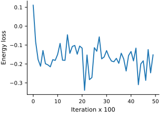
Let’s look at the evolution of the energy functional during training:

fig, ax = plt.subplots(figsize=FIGURE_SIZES["half_standard"])
ax.plot(losses)
ax.set_xlabel('Iteration x 100')
ax.set_ylabel('Energy loss')
finalize_axes(keep_box=False)

array([<Axes: xlabel='Iteration x 100', ylabel='Energy loss'>],
      dtype=object)

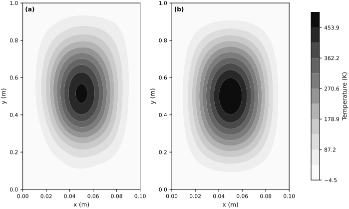
Panel (a) shows the neural approximation and panel (b) the exact temperature field. Both use the same grayscale range and colorbar.

u_true = u0 * jnp.sin(jnp.pi * X / Lx) ** 2 * jnp.sin(jnp.pi * Y / Ly) ** 2

vtu = jit(vmap(lambda xt, yt: ut(xt, yt, trained_model)))
u_pred = vtu(Xt_flat, Yt_flat).reshape(X.shape) * us

levels = np.linspace(float(jnp.minimum(u_pred.min(), u_true.min())),
                     float(jnp.maximum(u_pred.max(), u_true.max())), 12)
fig, axes = plt.subplots(1, 2, figsize=FIGURE_SIZES["full_landscape"], layout="constrained")
for ax, values in zip(axes, [u_pred, u_true]):
    contour = ax.contourf(X, Y, values, cmap="Greys", levels=levels)
    ax.set_xlabel("x (m)")
    ax.set_ylabel("y (m)")
label_panels(axes)
fig.colorbar(contour, ax=axes, label="Temperature (K)", shrink=0.9, pad=0.06)
finalize_axes(axes, keep_box=True)
plt.show()

findfont: Failed to find font weight semibold, now using 700.

fig, ax = plt.subplots(figsize=FIGURE_SIZES["full_tall"])
ax.set_xlabel(r'$\tilde{x}$')
ax.set_ylabel(r'$\tilde{y}$')
c = ax.contourf(to_xt(X), to_yt(Y), jnp.abs(u_pred - u_true), cmap='Greys')
plt.colorbar(c, ax=ax, label="Absolute temperature error (K)")
finalize_axes(keep_box=True)

array([<Axes: xlabel='$\\tilde{x}$', ylabel='$\\tilde{y}$'>,
       <Axes: label='<colorbar>', ylabel='Absolute temperature error (K)'>],
      dtype=object)

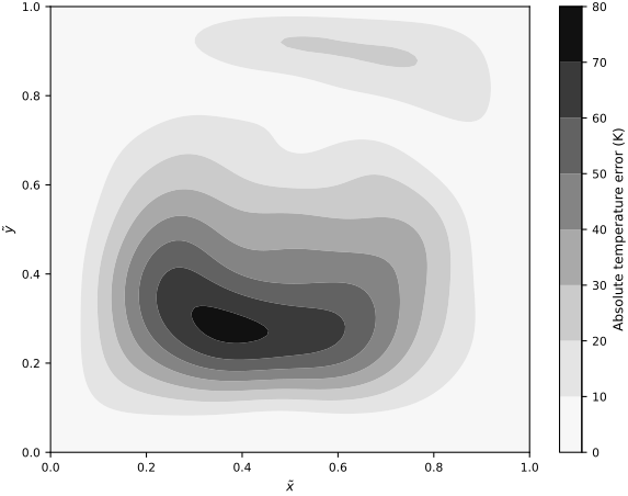
The error plot measures this finite training run. Accuracy depends on the network, collocation samples, and optimization budget; the energy formulation alone does not guarantee a more accurate neural approximation than residual minimization.