Polynomial Chaos in Many Dimensions

Polynomial Chaos in Many Dimensions#

Assume that we have a random vector:

\[ \Xi = (\Xi_1, \dots,\Xi_d), \]

where \(\Xi_i\) are independent random variables. The space of interest is the space of square-integrable functions on the probability space of \(\Xi\):

\[ L^2(\Xi) = \left\{ f : \mathbb{R}^d \to \mathbb{R} \mid \int_{\mathbb{R}^d} f(\xi)^2 \, d\mathbb{P}(\xi) < \infty \right\}. \]

To build an orthonormal basis in \(L^2(\Xi)\), we exploit the fact that:

\[ L^2(\Xi) = L^2(\Xi_1) \otimes \dots \otimes L^2(\Xi_d), \]

where the equality is understood as an isomorphism of Hilbert spaces. We can then build an orthonormal basis in \(L^2(\Xi)\) by taking the tensor product of univariate orthonormal bases in \(L^2(\Xi_i)\).

Using the multi-index notation, we can write the basis as:

\[ \left\{ \phi_\alpha(\xi) = \prod_{i=1}^d \phi_{\alpha_i}(\xi_i) \mid \alpha \in \mathbb{N}^d_0\right\}, \]

where \(\phi_{\alpha_i}\) is the univariate orthonormal basis in \(L^2(\Xi_i)\).

Typically, we need to truncate the basis to a finite number of terms. This is done by choosing a maximum degree \(p\) and taking only the multi-indices \(\alpha\) such that \(|\alpha|=\alpha_1+\dots+\alpha_d\leq p\). The truncated basis is then:

\[ \left\{ \phi_\alpha(\xi) = \prod_{i=1}^d \phi_{\alpha_i}(\xi_i) \mid \alpha \in \mathbb{N}^d_0, |\alpha| \leq p \right\}. \]

Example: Legendre polynomials in 2D#

Let us consider the case where \(\Xi_1\) and \(\Xi_2\) are independent uniform random variables in \([-1,1]\). Here is how we can construct the basis in \(L^2(\Xi)\):

import orthojax as ojax

degree1 = 3
phi1 = ojax.make_legendre_polynomial(degree1)
degree2 = 3
phi2 = ojax.make_legendre_polynomial(degree2)

total_degree = 6
phi = ojax.TensorProduct(total_degree, [phi1, phi2])

With each marginal family capped at degree three, this construction contains 16 products. The total-degree ceiling of six includes every pair of degrees allowed by these marginal caps. Here are the terms used to construct the basis:

print(f"Number of basis functions: {phi.num_basis}")
print("Terms in truncated tensor product:")
for i in range(phi.num_basis):
  print(f"ψ{i} = φ1{phi.terms[i][0]}⊗φ2{phi.terms[i][1]}")

Number of basis functions: 16
Terms in truncated tensor product:
ψ0 = φ10⊗φ20
ψ1 = φ11⊗φ20
ψ2 = φ10⊗φ21
ψ3 = φ12⊗φ20
ψ4 = φ11⊗φ21
ψ5 = φ10⊗φ22
ψ6 = φ13⊗φ20
ψ7 = φ12⊗φ21
ψ8 = φ11⊗φ22
ψ9 = φ10⊗φ23
ψ10 = φ13⊗φ21
ψ11 = φ12⊗φ22
ψ12 = φ11⊗φ23
ψ13 = φ13⊗φ22
ψ14 = φ12⊗φ23
ψ15 = φ13⊗φ23

You can evaluate it as follows:

import numpy as np

xs = np.random.randn(100, 2)
phis = phi(xs)
print(phis.shape)

(100, 16)

Let’s plot the first few basis functions:

x1 = np.linspace(-1, 1, 100)
x2 = np.linspace(-1, 1, 100)
X1, X2 = np.meshgrid(x1, x2)
X = np.stack([X1, X2], axis=-1)
X_flat = np.reshape(X, [-1, 2])
phis = phi(X_flat)
Z = np.reshape(phis, [100, 100, phi.num_basis])

for i in range(phi.num_basis):
  fig, ax = plt.subplots(figsize=FIGURE_SIZES["half_tall"])
  ax.contourf(X1, X2, Z[:, :, i], levels=20)

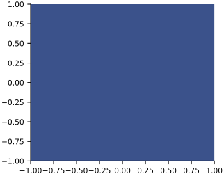
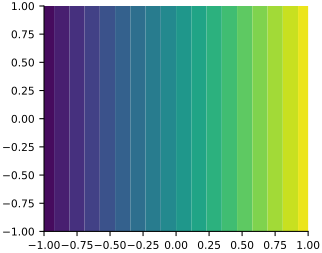
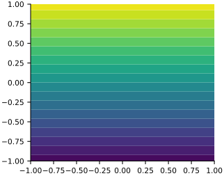
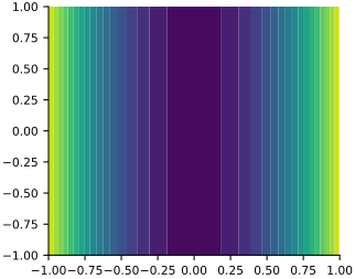
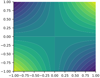
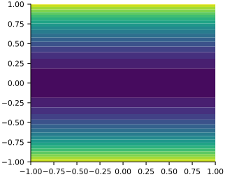
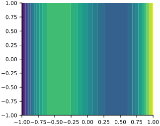
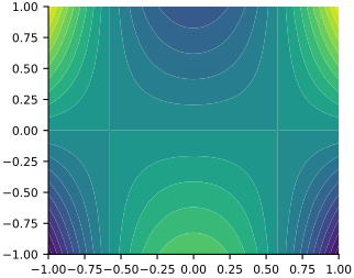
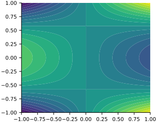
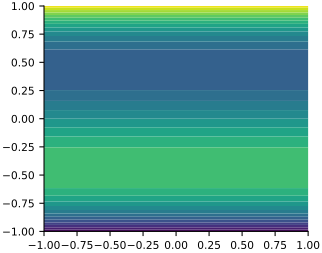
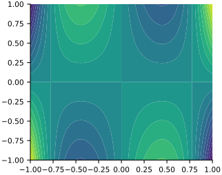
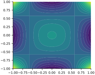
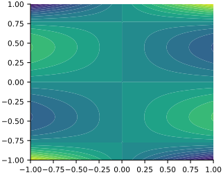
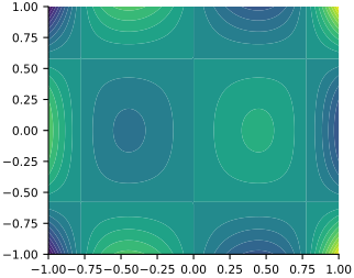
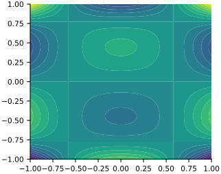
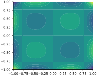
Let’s verify orthogonality. We need a quadrature rule in 2D. The simplest one is the tensor product of 1D quadrature rules. This would work, but it results to way to many quadrature points and it is not going to work in higher dimensions.

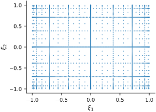
Instead, we use Smolyak sparse-grid quadrature (Smolyak, 1963). This is a quadrature rule that is based on a tensor product of nested 1D quadrature rules, but it only uses a subset of the tensor product. Nested quadrature rules are quadrature rules that are nested in the sense that the quadrature points of a rule of level \(\ell\) are a subset of the quadrature points of a rule of order \(\ell+1\).

Here is the Smolyak sparse grid quadrature rule of level 5 in 2D so that you can integrate the Legendre polynomials:

import design

num_dim = 2
level = 7
xs, ws = design.sparse_grid(num_dim, level, 'F1')
# Normalize the py-design weights for the uniform probability measure.
ws = ws / (2 ** num_dim)

Here are the quadrature points:

fig, ax = plt.subplots(figsize=FIGURE_SIZES["half_standard"])
ax.plot(xs[:, 0], xs[:, 1], '.', ms=1)
ax.set_xlabel("$\\xi_1$")
ax.set_ylabel("$\\xi_2$");

Two-dimensional sparse-grid quadrature nodes in the Legendre input domain.

Here is how we can do the inner products:

phis = phi(xs)
for i in range(phi.num_basis):
    for j in range(i, phi.num_basis):
        dot_ij = np.einsum("i,i,i->", ws, phis[:, i], phis[:, j])
        print(f"<ψ{i},ψ{j}> \t= {dot_ij:.3f}")

<ψ0,ψ0> 	= 1.000
<ψ0,ψ1> 	= -0.000
<ψ0,ψ2> 	= -0.000
<ψ0,ψ3> 	= 0.000
<ψ0,ψ4> 	= 0.000
<ψ0,ψ5> 	= 0.000
<ψ0,ψ6> 	= -0.000
<ψ0,ψ7> 	= 0.000
<ψ0,ψ8> 	= 0.000
<ψ0,ψ9> 	= -0.000
<ψ0,ψ10> 	= -0.000
<ψ0,ψ11> 	= -0.031
<ψ0,ψ12> 	= -0.000
<ψ0,ψ13> 	= -0.000
<ψ0,ψ14> 	= -0.000
<ψ0,ψ15> 	= 0.000
<ψ1,ψ1> 	= 1.000
<ψ1,ψ2> 	= -0.000
<ψ1,ψ3> 	= -0.000
<ψ1,ψ4> 	= -0.000
<ψ1,ψ5> 	= -0.000
<ψ1,ψ6> 	= -0.000
<ψ1,ψ7> 	= -0.000
<ψ1,ψ8> 	= -0.028
<ψ1,ψ9> 	= 0.000
<ψ1,ψ10> 	= -0.000
<ψ1,ψ11> 	= 0.000
<ψ1,ψ12> 	= -0.000
<ψ1,ψ13> 	= -0.032
<ψ1,ψ14> 	= -0.000
<ψ1,ψ15> 	= -0.000
<ψ2,ψ2> 	= 1.000
<ψ2,ψ3> 	= -0.000
<ψ2,ψ4> 	= -0.000
<ψ2,ψ5> 	= -0.000
<ψ2,ψ6> 	= 0.000
<ψ2,ψ7> 	= -0.028
<ψ2,ψ8> 	= -0.000
<ψ2,ψ9> 	= -0.000
<ψ2,ψ10> 	= -0.000
<ψ2,ψ11> 	= 0.000
<ψ2,ψ12> 	= -0.000
<ψ2,ψ13> 	= -0.000
<ψ2,ψ14> 	= -0.032
<ψ2,ψ15> 	= -0.000
<ψ3,ψ3> 	= 1.000
<ψ3,ψ4> 	= 0.000
<ψ3,ψ5> 	= -0.031
<ψ3,ψ6> 	= 0.000
<ψ3,ψ7> 	= -0.000
<ψ3,ψ8> 	= 0.000
<ψ3,ψ9> 	= -0.000
<ψ3,ψ10> 	= -0.000
<ψ3,ψ11> 	= -0.025
<ψ3,ψ12> 	= 0.000
<ψ3,ψ13> 	= -0.000
<ψ3,ψ14> 	= -0.000
<ψ3,ψ15> 	= 0.000
<ψ4,ψ4> 	= 0.975
<ψ4,ψ5> 	= 0.000
<ψ4,ψ6> 	= 0.000
<ψ4,ψ7> 	= -0.000
<ψ4,ψ8> 	= -0.000
<ψ4,ψ9> 	= 0.000
<ψ4,ψ10> 	= -0.029
<ψ4,ψ11> 	= 0.000
<ψ4,ψ12> 	= -0.029
<ψ4,ψ13> 	= 0.000
<ψ4,ψ14> 	= 0.000
<ψ4,ψ15> 	= -0.026
<ψ5,ψ5> 	= 1.000
<ψ5,ψ6> 	= -0.000
<ψ5,ψ7> 	= 0.000
<ψ5,ψ8> 	= -0.000
<ψ5,ψ9> 	= 0.000
<ψ5,ψ10> 	= 0.000
<ψ5,ψ11> 	= -0.025
<ψ5,ψ12> 	= -0.000
<ψ5,ψ13> 	= -0.000
<ψ5,ψ14> 	= -0.000
<ψ5,ψ15> 	= 0.000
<ψ6,ψ6> 	= 1.000
<ψ6,ψ7> 	= -0.000
<ψ6,ψ8> 	= -0.032
<ψ6,ψ9> 	= 0.000
<ψ6,ψ10> 	= -0.000
<ψ6,ψ11> 	= -0.000
<ψ6,ψ12> 	= -0.000
<ψ6,ψ13> 	= -0.044
<ψ6,ψ14> 	= -0.000
<ψ6,ψ15> 	= -0.000
<ψ7,ψ7> 	= 0.978
<ψ7,ψ8> 	= 0.000
<ψ7,ψ9> 	= -0.032
<ψ7,ψ10> 	= 0.000
<ψ7,ψ11> 	= -0.000
<ψ7,ψ12> 	= 0.000
<ψ7,ψ13> 	= 0.000
<ψ7,ψ14> 	= -0.019
<ψ7,ψ15> 	= -0.000
<ψ8,ψ8> 	= 0.978
<ψ8,ψ9> 	= -0.000
<ψ8,ψ10> 	= 0.000
<ψ8,ψ11> 	= -0.000
<ψ8,ψ12> 	= 0.000
<ψ8,ψ13> 	= -0.019
<ψ8,ψ14> 	= 0.000
<ψ8,ψ15> 	= -0.000
<ψ9,ψ9> 	= 1.000
<ψ9,ψ10> 	= -0.000
<ψ9,ψ11> 	= -0.000
<ψ9,ψ12> 	= -0.000
<ψ9,ψ13> 	= -0.000
<ψ9,ψ14> 	= -0.044
<ψ9,ψ15> 	= -0.000
<ψ10,ψ10> 	= 0.961
<ψ10,ψ11> 	= 0.000
<ψ10,ψ12> 	= -0.026
<ψ10,ψ13> 	= -0.000
<ψ10,ψ14> 	= -0.000
<ψ10,ψ15> 	= -0.044
<ψ11,ψ11> 	= 0.987
<ψ11,ψ12> 	= 0.000
<ψ11,ψ13> 	= 0.000
<ψ11,ψ14> 	= 0.000
<ψ11,ψ15> 	= -0.000
<ψ12,ψ12> 	= 0.961
<ψ12,ψ13> 	= -0.000
<ψ12,ψ14> 	= -0.000
<ψ12,ψ15> 	= -0.044
<ψ13,ψ13> 	= 0.966
<ψ13,ψ14> 	= 0.000
<ψ13,ψ15> 	= 0.000
<ψ14,ψ14> 	= 0.966
<ψ14,ψ15> 	= 0.000
<ψ15,ψ15> 	= 0.939

You want the level high enough so that these are accurate to some extent. This looks correct.

Example: Hermite polynomials in 2D#

Let’s do the same thing for normal random variables. Here \(\Xi_1\) and \(\Xi_2\) are independent standard normal random variables and \(\Xi = (\Xi_1, \Xi_2)\).

Make the polynomials:

degree1 = 3
phi1 = ojax.make_hermite_polynomial(degree1)
degree2 = 3
phi2 = ojax.make_hermite_polynomial(degree2)

total_degree = 6
phi = ojax.TensorProduct(total_degree, [phi1, phi2])

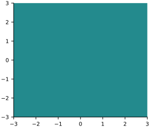
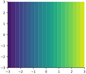
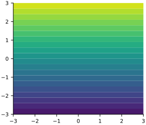
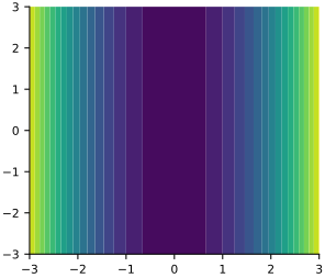
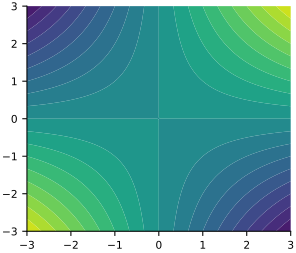
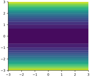
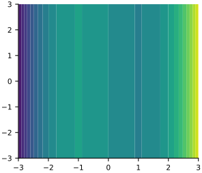
Let’s plot them:

x1 = np.linspace(-3, 3, 100)
x2 = np.linspace(-3, 3, 100)
X1, X2 = np.meshgrid(x1, x2)
X = np.stack([X1, X2], axis=-1)
X_flat = np.reshape(X, [-1, 2])
phis = phi(X_flat)
Z = np.reshape(phis, [100, 100, phi.num_basis])

for i in range(phi.num_basis):
  fig, ax = plt.subplots(figsize=FIGURE_SIZES["half_tall"])
  ax.contourf(X1, X2, Z[:, :, i], levels=20)

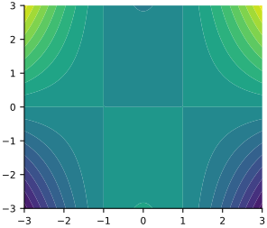
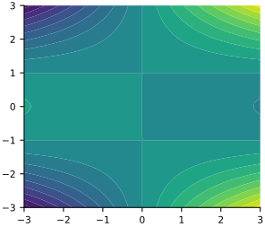
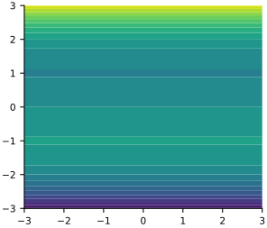
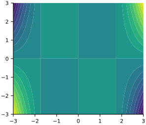
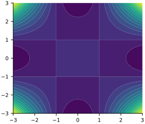
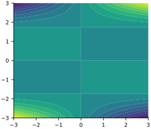
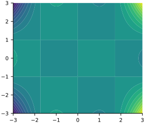
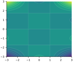
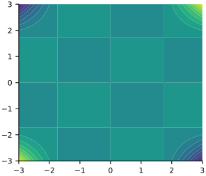
Sixteen contour maps of the two-dimensional tensor-product Hermite basis functions, ranging from the constant mode to progressively higher polynomial variation in each coordinate.

Let’s test orthogonality. Here we need also a sparse grid but for Hermite polynomials.

num_dim = 2
level = 6
xs, ws = design.sparse_grid(num_dim, level, 'GH') # Notice that I changed CC to GH
# Normalize the py-design weights for the standard normal measure.
xs = xs * np.sqrt(2)
ws = ws / np.sqrt(np.pi ** num_dim)

phis = phi(xs)
for i in range(phi.num_basis):
    for j in range(i, phi.num_basis):
        dot_ij = np.einsum("i,i,i->", ws, phis[:, i], phis[:, j])
        print(f"<ψ{i},ψ{j}> \t= {dot_ij:.3f}")

<ψ0,ψ0> 	= 1.000
<ψ0,ψ1> 	= -0.000
<ψ0,ψ2> 	= -0.000
<ψ0,ψ3> 	= 0.000
<ψ0,ψ4> 	= 0.000
<ψ0,ψ5> 	= 0.000
<ψ0,ψ6> 	= -0.000
<ψ0,ψ7> 	= 0.000
<ψ0,ψ8> 	= 0.000
<ψ0,ψ9> 	= -0.000
<ψ0,ψ10> 	= -0.000
<ψ0,ψ11> 	= 0.000
<ψ0,ψ12> 	= -0.000
<ψ0,ψ13> 	= -0.000
<ψ0,ψ14> 	= -0.000
<ψ0,ψ15> 	= -0.000
<ψ1,ψ1> 	= 1.000
<ψ1,ψ2> 	= 0.000
<ψ1,ψ3> 	= -0.000
<ψ1,ψ4> 	= -0.000
<ψ1,ψ5> 	= -0.000
<ψ1,ψ6> 	= -0.000
<ψ1,ψ7> 	= -0.000
<ψ1,ψ8> 	= 0.000
<ψ1,ψ9> 	= 0.000
<ψ1,ψ10> 	= 0.000
<ψ1,ψ11> 	= -0.000
<ψ1,ψ12> 	= -0.000
<ψ1,ψ13> 	= -0.000
<ψ1,ψ14> 	= -0.000
<ψ1,ψ15> 	= -0.000
<ψ2,ψ2> 	= 1.000
<ψ2,ψ3> 	= -0.000
<ψ2,ψ4> 	= -0.000
<ψ2,ψ5> 	= -0.000
<ψ2,ψ6> 	= 0.000
<ψ2,ψ7> 	= 0.000
<ψ2,ψ8> 	= -0.000
<ψ2,ψ9> 	= -0.000
<ψ2,ψ10> 	= -0.000
<ψ2,ψ11> 	= -0.000
<ψ2,ψ12> 	= 0.000
<ψ2,ψ13> 	= -0.000
<ψ2,ψ14> 	= -0.000
<ψ2,ψ15> 	= -0.000
<ψ3,ψ3> 	= 1.000
<ψ3,ψ4> 	= 0.000
<ψ3,ψ5> 	= 0.000
<ψ3,ψ6> 	= 0.000
<ψ3,ψ7> 	= -0.000
<ψ3,ψ8> 	= -0.000
<ψ3,ψ9> 	= -0.000
<ψ3,ψ10> 	= -0.000
<ψ3,ψ11> 	= 0.000
<ψ3,ψ12> 	= -0.000
<ψ3,ψ13> 	= -0.000
<ψ3,ψ14> 	= -0.000
<ψ3,ψ15> 	= 0.000
<ψ4,ψ4> 	= 1.000
<ψ4,ψ5> 	= 0.000
<ψ4,ψ6> 	= 0.000
<ψ4,ψ7> 	= -0.000
<ψ4,ψ8> 	= -0.000
<ψ4,ψ9> 	= 0.000
<ψ4,ψ10> 	= -0.000
<ψ4,ψ11> 	= -0.000
<ψ4,ψ12> 	= -0.000
<ψ4,ψ13> 	= 0.000
<ψ4,ψ14> 	= 0.000
<ψ4,ψ15> 	= -0.000
<ψ5,ψ5> 	= 1.000
<ψ5,ψ6> 	= -0.000
<ψ5,ψ7> 	= -0.000
<ψ5,ψ8> 	= -0.000
<ψ5,ψ9> 	= 0.000
<ψ5,ψ10> 	= -0.000
<ψ5,ψ11> 	= 0.000
<ψ5,ψ12> 	= -0.000
<ψ5,ψ13> 	= -0.000
<ψ5,ψ14> 	= -0.000
<ψ5,ψ15> 	= 0.000
<ψ6,ψ6> 	= 1.000
<ψ6,ψ7> 	= -0.000
<ψ6,ψ8> 	= -0.000
<ψ6,ψ9> 	= 0.000
<ψ6,ψ10> 	= -0.000
<ψ6,ψ11> 	= -0.000
<ψ6,ψ12> 	= -0.000
<ψ6,ψ13> 	= 0.000
<ψ6,ψ14> 	= -0.000
<ψ6,ψ15> 	= -0.000
<ψ7,ψ7> 	= 1.000
<ψ7,ψ8> 	= -0.000
<ψ7,ψ9> 	= -0.000
<ψ7,ψ10> 	= 0.000
<ψ7,ψ11> 	= -0.000
<ψ7,ψ12> 	= 0.000
<ψ7,ψ13> 	= -0.000
<ψ7,ψ14> 	= -0.000
<ψ7,ψ15> 	= -0.000
<ψ8,ψ8> 	= 1.000
<ψ8,ψ9> 	= -0.000
<ψ8,ψ10> 	= 0.000
<ψ8,ψ11> 	= -0.000
<ψ8,ψ12> 	= 0.000
<ψ8,ψ13> 	= -0.000
<ψ8,ψ14> 	= -0.000
<ψ8,ψ15> 	= -0.000
<ψ9,ψ9> 	= 1.000
<ψ9,ψ10> 	= -0.000
<ψ9,ψ11> 	= -0.000
<ψ9,ψ12> 	= -0.000
<ψ9,ψ13> 	= -0.000
<ψ9,ψ14> 	= 0.000
<ψ9,ψ15> 	= -0.000
<ψ10,ψ10> 	= 1.000
<ψ10,ψ11> 	= -0.000
<ψ10,ψ12> 	= 0.000
<ψ10,ψ13> 	= -0.000
<ψ10,ψ14> 	= -0.000
<ψ10,ψ15> 	= -0.000
<ψ11,ψ11> 	= 1.000
<ψ11,ψ12> 	= -0.000
<ψ11,ψ13> 	= 0.000
<ψ11,ψ14> 	= 0.000
<ψ11,ψ15> 	= -0.000
<ψ12,ψ12> 	= 1.000
<ψ12,ψ13> 	= -0.000
<ψ12,ψ14> 	= -0.000
<ψ12,ψ15> 	= -0.000
<ψ13,ψ13> 	= 1.000
<ψ13,ψ14> 	= -0.000
<ψ13,ψ15> 	= 0.000
<ψ14,ψ14> 	= 1.000
<ψ14,ψ15> 	= 0.000
<ψ15,ψ15> 	= 1.000

Dealing with a mix of random variables#

Above we had either only uniform or only normal random variables. If you have mixed versions, you have two choices:

Map all random variables to uniform and use the recipe above. You can do this as follows. Take \(\Xi_i\) following a distribution with cumulative distribution function (CDF) \(F_i\). Then \(\Xi_i = F_i^{-1}(U_i)\), where \(U_i\) is a uniform random variable in \([0,1]\). Then work with \(U_i\).
Keep each variable’s own orthonormal polynomial family and integrate with a sparse-grid quadrature rule built from tensor products of nested one-dimensional rules matched to each variable. This construction is due to Smolyak (Smolyak, 1963); software packages such as Chaospy provide implementations, although they are not JAX-native.

Dealing with Random Variables that are Not Independent#

If you have a multivariate normal:

\[ \Xi \sim \mathcal{N}(\mu, \Sigma), \]

you can use the fact that:

\[ \Xi = \mu + L Z, \]

where

\[ \Sigma = L L^{\mathsf T}, \]

and \(Z\) is a vector of independent standard normal random variables. Furthermore, you can go to uniform random variables by using the CDF of the normal distribution. That is, we can write:

\[ \Xi = \mu + L \Phi^{-1}(U), \]

where \(\Phi\) is the standard normal CDF applied componentwise and \(U\) is a vector of independent uniform random variables in \([0,1]\).

For a more general joint distribution, the Rosenblatt transformation maps the dependent variables to independent uniform variables through conditional cumulative distribution functions (Rosenblatt, 1952).