

Example: Gaussian Process Regression with Large Data Sets#
An autoinjector is an automated injection device that inserts a needle and delivers a drug beneath the skin. The simulator of Sree et al. (2023) varies ten drug, device, and tissue inputs, including viscosity, needle size, and tissue properties. We use 10,000 simulations to predict the needle insertion depth at the onset of drug delivery and reserve 500 different simulations for testing. The purpose is to show how the inducing-variable construction from the preceding section turns a dense Gaussian process into a bounded computation, and then to assess the resulting predictions on data that played no role in fitting.
The implementation uses GPJax (Pinder and Dodd, 2022). We model one response so that the computational and statistical diagnostics remain visible; the same workflow can be repeated separately for the other outputs.
Data and preprocessing#
The training and test data are stored in separate files. All centering and scaling constants are computed from the training data and then applied unchanged to the test data. We leave the rows in their stored order; the optimization routine draws reproducible minibatches from a fixed JAX random key.
INPUT_COLUMNS = [
    "mu", "fill_volume", "hGap0", "lNeedle", "dNeedle",
    "FSpring0", "kSpring", "kappa5", "kappa6", "kappa7",
]
OUTPUT_COLUMN = "Needle displacement (m)"

train = load_workbook("training_data.xlsx")
test = load_workbook("test_data.xlsx")

X_train_raw = train[INPUT_COLUMNS].to_numpy(dtype=float)
y_train_raw = train[[OUTPUT_COLUMN]].to_numpy(dtype=float)
X_test_raw = test[INPUT_COLUMNS].to_numpy(dtype=float)
y_test_raw = test[[OUTPUT_COLUMN]].to_numpy(dtype=float)

assert X_train_raw.shape == (10_000, 10)
assert X_test_raw.shape == (500, 10)
training_inputs = {tuple(row) for row in X_train_raw}
assert not any(tuple(row) in training_inputs for row in X_test_raw)

X_mean, X_std = X_train_raw.mean(axis=0), X_train_raw.std(axis=0)
y_mean, y_std = y_train_raw.mean(axis=0), y_train_raw.std(axis=0)

X_train = jnp.asarray((X_train_raw - X_mean) / X_std)
X_test = jnp.asarray((X_test_raw - X_mean) / X_std)
y_train = jnp.asarray((y_train_raw - y_mean) / y_std)
y_test = jnp.asarray((y_test_raw - y_mean) / y_std)

print(f"Training cases: {X_train.shape[0]:,}")
print(f"Independent test cases: {X_test.shape[0]:,}")
Training cases: 10,000
Independent test cases: 500
Computational limits of a dense exact GP#
An exact GP at \(n=10{,}000\) training inputs requires a dense \(n\times n\) covariance matrix. That matrix alone contains \(10^8\) entries, or \(0.80\) GB in double precision, before the factorization workspace and intermediate arrays are counted. A dense Cholesky factorization has leading cost \(n^3/3\approx 3.3\times 10^{11}\) floating-point operations each time the covariance parameters change. We therefore do not attempt the dense exact fit. These figures are algebraic resource estimates, not timing measurements.
For the stochastic variational GP below, let \(m=128\) be the number of inducing inputs and \(b=256\) the minibatch size. A training update has leading algebraic cost \(\mathcal{O}(m^3+bm^2)\) and works with matrices whose dimensions are governed by \(m\) and \(b\), rather than by all \(n\) observations at once.
A reproducible inducing-input initialization#
The inducing matrix \(Z\) should represent the observed ten-dimensional input cloud. The following deterministic farthest-point traversal selects actual standardized training rows. It starts near the center of the data and repeatedly adds the row farthest from the current set. This is a reproducible, space-filling initialization in standardized Euclidean distance, not a claim that the selected set is optimal.
def farthest_point_subset(X, number):
    X = np.asarray(X)
    indices = np.empty(number, dtype=int)
    indices[0] = np.argmin(np.sum((X - X.mean(axis=0)) ** 2, axis=1))
    nearest_squared_distance = np.sum((X - X[indices[0]]) ** 2, axis=1)

    for k in range(1, number):
        indices[k] = np.argmax(nearest_squared_distance)
        candidate_distance = np.sum((X - X[indices[k]]) ** 2, axis=1)
        nearest_squared_distance = np.minimum(
            nearest_squared_distance, candidate_distance
        )
    return indices


number_of_inducing_inputs = 128
inducing_indices = farthest_point_subset(X_train, number_of_inducing_inputs)
Z = X_train[inducing_indices]
Inducing matrix Z: (128, 10)
Variational model and objective#
The code uses a zero-mean GP with an automatic-relevance-determination radial-basis-function kernel and a Gaussian likelihood. The object named q represents the variational distribution \(q(\mathbf{u})\) at inducing_inputs=Z. A whitened parameterization improves numerical conditioning.
For fixed covariance parameters, likelihood parameters, and inducing inputs, maximizing the ELBO is equivalent to minimizing the corresponding Kullback–Leibler divergence up to the constant log evidence. Here those model parameters and \(Z\) are optimized jointly with the variational parameters, so the ELBO is the joint training criterion. It is not a substitute for test-set validation. Unlike the exact marginal log likelihood, the likelihood-expectation term in this uncollapsed ELBO is additive over observations; GPJax applies the \(n/b\) scaling derived in the preceding section when it evaluates a minibatch.
data = gpx.Dataset(X=X_train, y=y_train)

prior = gpx.gps.Prior(
    mean_function=gpx.mean_functions.Zero(),
    kernel=gpx.kernels.RBF(
        lengthscale=jnp.ones(X_train.shape[1]),
        variance=1.0,
    ),
)
likelihood = gpx.likelihoods.Gaussian(
    num_datapoints=data.n,
    obs_stddev=0.1,
)
posterior = prior * likelihood

q = gpx.variational_families.WhitenedVariationalGaussian(
    posterior=posterior,
    inducing_inputs=Z,
)
negative_elbo = jax.jit(
    lambda model, batch: -gpx.objectives.elbo(model, batch)
)
number_of_steps = 10_000
minibatch_size = 256

q, loss_history = gpx.fit(
    model=q,
    objective=negative_elbo,
    train_data=data,
    optim=optax.adam(learning_rate=5e-3),
    num_iters=number_of_steps,
    batch_size=minibatch_size,
    key=jr.key(2026),
    verbose=False,
    safe=True,
)
loss_history.block_until_ready();
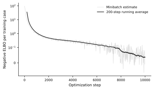
The optimization history is the negative minibatch ELBO, divided by the number of training observations. Its stochastic fluctuations are expected. The running average shows the long-term trend, but neither curve establishes predictive accuracy; that assessment uses the independent test cases.
loss_per_case = np.asarray(loss_history) / data.n
window = 200
running_average = np.convolve(
    loss_per_case, np.ones(window) / window, mode="valid"
)

fig, ax = plt.subplots(figsize=(5.2, 3.0), constrained_layout=True)
steps = np.arange(1, number_of_steps + 1)
ax.plot(
    steps[::20], loss_per_case[::20],
    color=BOOK_COLORS["light"], linewidth=0.8, label="Minibatch estimate",
)
ax.plot(
    steps[window - 1 :], running_average,
    color=BOOK_COLORS["dark"], label=f"{window}-step running average",
)
ax.set_yscale("symlog", linthresh=0.1)
ax.set_xlabel("Optimization step")
ax.set_ylabel("Negative ELBO per training case")
ax.legend()
plt.show()
Independent predictive assessment#
GPJax forms a joint Gaussian distribution for the requested prediction inputs. We request only 100 test points at a time so that the size of this joint distribution remains bounded. Applying the Gaussian likelihood adds the fitted observation-model nugget to the latent uncertainty. For these deterministic simulator outputs, that nugget should be interpreted as unresolved model discrepancy and numerical regularization, not as intrinsic experimental randomness.
def predictive_marginals(model, X, chunk_size=100):
    means, standard_deviations = [], []
    for start in range(0, X.shape[0], chunk_size):
        latent_distribution = model(X[start : start + chunk_size])
        predictive_distribution = model.posterior.likelihood(latent_distribution)
        means.append(np.asarray(predictive_distribution.mean).reshape(-1))
        standard_deviations.append(
            np.asarray(predictive_distribution.stddev()).reshape(-1)
        )
    return np.concatenate(means), np.concatenate(standard_deviations)


predictive_mean, predictive_std = predictive_marginals(q, X_test)
test_values = np.asarray(y_test).reshape(-1)
standardized_residual = (test_values - predictive_mean) / predictive_std

rmse_scaled = np.sqrt(np.mean((predictive_mean - test_values) ** 2))
rmse_mm = float(rmse_scaled * y_std[0] * 1_000)
nlpd_scaled = np.mean(
    0.5 * np.log(2 * np.pi * predictive_std**2)
    + 0.5 * standardized_residual**2
)
coverage_68 = np.mean(np.abs(standardized_residual) <= 1.0)
coverage_95 = np.mean(np.abs(standardized_residual) <= 1.96)

print(f"Test RMSE: {rmse_mm:.3f} mm")
print(f"Test negative log predictive density (standardized): {nlpd_scaled:.3f}")
print(
    "Standardized residual mean / standard deviation: "
    f"{standardized_residual.mean():.3f} / {standardized_residual.std():.3f}"
)
print(f"Central 68% / 95% interval coverage: {coverage_68:.1%} / {coverage_95:.1%}")
Test RMSE: 0.825 mm
Test negative log predictive density (standardized): -0.073
Standardized residual mean / standard deviation: -0.003 / 0.886
Central 68% / 95% interval coverage: 79.0% / 94.2%
true_mm = (test_values * y_std[0] + y_mean[0]) * 1_000
mean_mm = (predictive_mean * y_std[0] + y_mean[0]) * 1_000

nominal_coverage = np.linspace(0.10, 0.99, 60)
critical_values = norm.ppf((1.0 + nominal_coverage) / 2.0)
empirical_coverage = np.array(
    [np.mean(np.abs(standardized_residual) <= value) for value in critical_values]
)

fig, axes = plt.subplots(1, 3, figsize=(7.35, 2.55), constrained_layout=True)

axes[0].scatter(
    true_mm, mean_mm, s=12, facecolors="white", edgecolors=BOOK_COLORS["dark"],
    linewidths=0.6,
)
limits = [min(true_mm.min(), mean_mm.min()), max(true_mm.max(), mean_mm.max())]
axes[0].plot(limits, limits, "--", color=BOOK_COLORS["medium"], label="Ideal")
axes[0].set(xlabel="Simulated displacement (mm)", ylabel="Predictive mean (mm)")
axes[0].text(
    0.96, 0.06, f"RMSE = {rmse_mm:.3f} mm",
    transform=axes[0].transAxes, ha="right", va="bottom",
)

grid = np.linspace(-4, 4, 300)
axes[1].hist(
    standardized_residual, bins=22, density=True,
    color="white", edgecolor=BOOK_COLORS["dark"], linewidth=0.8,
)
axes[1].plot(grid, norm.pdf(grid), "--", color=BOOK_COLORS["medium"], label=r"$\mathcal{N}(0,1)$")
axes[1].set(xlabel="Standardized residual", ylabel="Density")
axes[1].legend()

axes[2].plot(
    nominal_coverage, empirical_coverage,
    color=BOOK_COLORS["dark"], marker="o", markevery=8, markersize=3,
    label="Test data",
)
axes[2].plot([0, 1], [0, 1], "--", color=BOOK_COLORS["medium"], label="Ideal")
axes[2].set(
    xlim=(0, 1), ylim=(0, 1),
    xlabel="Nominal central coverage", ylabel="Empirical coverage",
)
axes[2].legend()

for label, ax in zip(["(a)", "(b)", "(c)"], axes):
    ax.text(0.02, 0.98, label, transform=ax.transAxes, va="top", fontweight="bold")

plt.show()
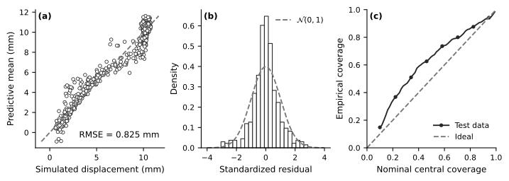
The independent test RMSE is about \(0.83\) mm. The 95% intervals attain coverage close to their nominal level, while the 68% intervals are conservative. The standardized residuals are nearly centered but are somewhat narrower than a standard normal distribution. The parity plot also exposes a few negative predictive means near the lower boundary, which are physically inadmissible and motivate a positive-output transformation when that constraint matters. Thus the model gives a useful first surrogate, but it is neither perfectly calibrated nor constraint preserving. This conclusion comes from the held-out simulations, not from the ELBO trace.
Exercise#
Repeat the fit with \(m\in\{64,128,256\}\) while keeping the data split, random key, minibatch size, optimizer, and stopping rule fixed. For each fit, record the independent-test RMSE, negative log predictive density, and 68% and 95% coverage. Then replace the farthest-point initialization by a seeded random subset of training inputs. Explain the observed changes without using the training ELBO alone, and relate the computational change to the \(\mathcal{O}(m^3+bm^2)\) training-update cost. Finally, test whether modeling the logarithm of the displacement removes the physically inadmissible negative predictions.