Population uncertainty

Population uncertainty#

Cars on a bumpy road#

There is a bump on the road that causes cars to oscillate after hitting it. The nature of the oscillation depends on the car’s mass and suspension system. You’ve installed a camera on the highway that can capture snapshots of each car’s vertical displacement. You capture 20 snapshots per car before they drive out of the camera’s view. Suppose you want to infer the cars’ suspension dynamics parameters (with uncertainty).

First, we need a forward model for the vertical displacement \(x\) of a car. We’ll model this as a damped harmonic oscillator

\[\begin{split} \begin{equation*} \begin{aligned} &\ddot{x} + 2\zeta\dot{x} + \omega^2 x = 0 \\ &x(0) = x_0 \\ &\dot{x}(0) = 0 \end{aligned} \end{equation*} \end{split}\]

where \(\zeta\) is the damping ratio and \(\omega\) is the natural frequency. Let \(x(t; x_0, \zeta, \omega)\) be the vertical position of a car at time \(t\), which is obtained by solving the above ordinary differential equation (ODE).

This ODE happens to have an analytic solution. Let’s code it up and visualize:

Show code cell source Hide code cell source

@jit
def damped_harmonic_oscillator(t, x0, v0, zeta, omega):
    """
    Computes the displacement x(t) of a damped harmonic oscillator.
    
    Parameters
    ----------
        t: Time (scalar or array).
        x0: Initial displacement.
        v0: Initial velocity.
        omega: Natural frequency (rad/s).
        zeta: Damping ratio.

    Returns:
        x: Displacement x(t) at time t.
    """
    kwargs = dict(x0=x0, v0=v0, omega=omega)
    index = jnp.where(zeta < 1.0, 0, jnp.where(jnp.isclose(zeta, 1.0), 1, 2))
    x = lax.switch(
        index,
        [partial(underdamped_solution, zeta=zeta, **kwargs), partial(critically_damped_solution, **kwargs), partial(overdamped_solution, zeta=zeta, **kwargs)],
        t
    )
    return x

def underdamped_solution(t, x0, v0, zeta, omega):
    omega_d = omega * jnp.sqrt(1 - zeta**2)  # Damped natural frequency
    A = x0
    B = (v0 + zeta * omega * x0) / omega_d  # From initial velocity
    x = jnp.exp(-zeta * omega * t) * (A * jnp.cos(omega_d * t) + B * jnp.sin(omega_d * t))
    return x

def critically_damped_solution(t, x0, v0, omega):
    A = x0
    B = v0 + omega * x0
    x = (A + B * t) * jnp.exp(-omega * t)
    return x

def overdamped_solution(t, x0, v0, zeta, omega):
    r1 = -omega * (zeta - jnp.sqrt(zeta**2 - 1))
    r2 = -omega * (zeta + jnp.sqrt(zeta**2 - 1))
    A = (v0 - r2 * x0) / (r1 - r2)
    B = (r1 * x0 - v0) / (r1 - r2)
    x = A * jnp.exp(r1 * t) + B * jnp.exp(r2 * t)
    return x

# Parameters
x0 = 1.0       # Initial displacement
v0 = 0.0       # Initial velocity
omega = 3.0  # Natural frequency (rad/s)
zetas = [0.1, 1.0, 10.0]  # Damping ratio

# Time array
t = jnp.linspace(0, 10, 500)

# Compute displacement and velocity
xs = [damped_harmonic_oscillator(t, x0, v0, zeta_i, omega) for zeta_i in zetas]
x_underdamped, x_critically_damped, x_overdamped = xs

fig, ax = plt.subplots(figsize=(7, 3))
ax.plot(t, x_underdamped, lw=2, label='underdamped')
ax.plot(t, x_critically_damped, lw=2, label='critically damped')
ax.plot(t, x_overdamped, lw=2, label='overdamped')
ax.axhline(0, color="black", lw=1, ls='--', zorder=-10)
ax.set_ylabel("Displacement")
ax.set_xlabel("Time")
ax.set_title("Damped Harmonic Oscillator")
ax.legend()
sns.despine(trim=True)

../../_images/2fa88945cce10f3d29edc1bbe39f598a77881379d0c6b2023b87c2f3bd07389e.svg

Hierarchical probabilistic model#

Population distribution#

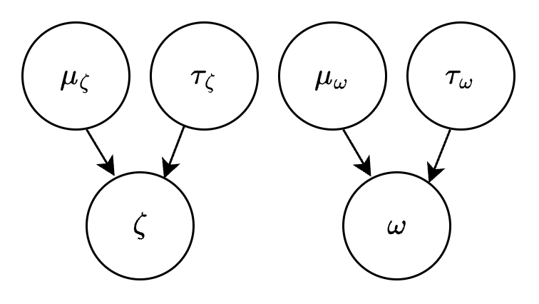
We want to answer the following question: For a random car, what is the prior distribution over its suspension dynamics parameters (i.e., damping ratio \(\zeta\) and natural frequency \(\omega\))?

In this context, the prior distribution is often called the population distribution. We write it as

\[\begin{split} \underbrace{p(\zeta, \omega)}_{\substack{\text{population} \\ \text{distribution}}} = \int \underbrace{p(\zeta, \omega | \theta_\text{pop})}_{\substack{\text{conditional} \\ \text{prior}}} \underbrace{p(\theta_\text{pop})}_{\substack{\text{prior on} \\ \text{population} \\ \text{parameters}}} d\theta_\text{pop} \end{split}\]

where \(\theta_\text{pop}\) are the population parameters. Let the conditional prior be defined with

\[\begin{split} \log \zeta | \mu_\zeta, \tau_\zeta \sim \text{Normal}(\mu_\zeta, \tau_\zeta^2) \\ \log \omega | \mu_\omega, \tau_\omega \sim \text{Normal}(\mu_\omega, \tau_\omega^2) \end{split}\]

where \(\mu_\zeta\) and \(\tau_\zeta\) are the population mean and standard deviation for \(\log \zeta\) (and similarly for \(\omega\)). The population parameters are then just

\[ \theta_\text{pop}=(\mu_\zeta, \tau_\zeta, \mu_\omega, \tau_\omega). \]

Let’s define the prior on these population parameters with

\[\begin{split} \begin{align*} \mu_\zeta &\sim \text{Normal}(-1, 1) \\ \tau_\zeta &\sim \text{Exponential}(10) \\ \mu_\omega &\sim \text{Normal}(0, 0.5) \\ \tau_\omega &\sim \text{Exponential}(10) \end{align*} \end{split}\]

This is the directed acyclic graph (DAG) associated with our model so far:

Connecting the population distribution to the data#

Suppose we observe 30 cars driving over the same bump. Let’s assume the initial displacement \(x_0\) is the same for all cars, and that it is between 0 and 5 inches:

\[ x_0 \sim \text{Uniform}([0, 5]) \]

Finally, let the observed displacement of car \(i\) at time \(j\) be

\[ y_{ij}| t_{ij}, \zeta_i, \omega_i, x_0 \sim \text{Normal}\Big(x(t_{ij}; x_0, \zeta_i, \omega_i), \sigma^2 \Big) \]

where the measurement noise \(\sigma\) is known. Here is the DAG for the full hierarchical model:

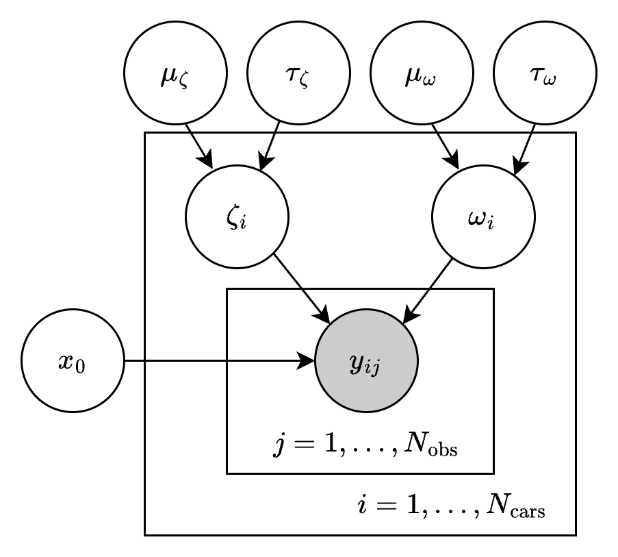
We can write down the posterior as

\[\begin{split} \begin{align*} p(\underbrace{\theta_\text{pop}, \zeta, \omega, x_0}_\text{unknowns}| \underbrace{\mathbf{t}, \mathbf{y}}_\text{data}) \propto \left[ \prod_{i=1}^{30} \left[ \prod_{j=1}^M \underbrace{p(y_{ij}|t_{ij}, \zeta_i, \omega_i, x_0, \sigma^2)}_\text{likelihood of an observation} \right] \underbrace{p(\zeta_i|\mu_\zeta, \tau_\zeta) ~ p(\omega_i|\mu_\omega, \tau_\omega)}_\text{conditional priors} \right] ~ \underbrace{p(\mu_\zeta) ~ p(\tau_\zeta) ~ p(\mu_\omega) ~ p(\tau_\omega)}_{\substack{\text{prior on} \\ \text{population parameters}}} \underbrace{p(x_0)}_{\substack{\text{initial condition} \\ \text{prior}}} \end{align*} \end{split}\]

where \(\zeta = (\zeta_1, \dots, \zeta_{30})\) and \(\omega = (\omega_1, \dots, \omega_{30})\) are the sets of physical parameters for all 30 cars in the dataset. Finally, we’ll transform all random variables to a single random vector \(\xi\) which lives in unconstrained space \(\mathbb{R}^d\).

Building the model with Numpyro#

We will use Numpyro to construct both the log probability density \(p(\xi|\mathbf{t}, \mathbf{y})\) and the transformation \(\xi \mapsto (\theta_\text{pop}, \zeta, \omega, x_0)\). First, let’s write the model using Numpyro objects:

N_TIMES = 20
N_INDIVIDUALS = 100
MEASUREMENT_NOISE = 0.1
PARAMETERIZATION = 'centered'
times = jnp.linspace(0, 4, N_TIMES)

if PARAMETERIZATION == 'centered':

    def model(obs, gamma, prior_only=False):
        # Population parameters
        mu_zeta = numpyro.sample("mu_zeta", dist.Normal(-2.0, 1.0))
        tau_zeta = numpyro.sample("tau_zeta", dist.Exponential(10.0))
        mu_omega = numpyro.sample("mu_omega", dist.Normal(0.0, 0.5))
        tau_omega = numpyro.sample("tau_omega", dist.Exponential(10.0))

        # Initial condition
        x0 = numpyro.sample("x0", dist.Uniform(0, 5))

        # Physical parameters
        with numpyro.plate("individuals", N_INDIVIDUALS):
            log_zeta = numpyro.sample("log_zeta", dist.Normal(mu_zeta, tau_zeta))
            log_omega = numpyro.sample("log_omega", dist.Normal(mu_omega, tau_omega))
            zeta = jnp.exp(log_zeta)
            omega = jnp.exp(log_omega)

            if not prior_only:
                # Solve the ODE
                solver = lambda zeta, omega: damped_harmonic_oscillator(t=times, x0=x0, v0=0.0, zeta=zeta, omega=omega)
                x = vmap(solver, out_axes=-1)(zeta, omega)

                # Observations
                with numpyro.plate("observations", N_TIMES):
                    with numpyro.handlers.scale(scale=gamma):
                        y = numpyro.sample("y", dist.Normal(x, MEASUREMENT_NOISE), obs=obs)
        
        return locals()  # Returns a dict of all locally-defined variables

if PARAMETERIZATION == 'noncentered':

    def model(obs, gamma, prior_only=False):
        # Population parameters
        mu_zeta = numpyro.sample("mu_zeta", dist.Normal(-2.0, 1.0))
        tau_zeta = numpyro.sample("tau_zeta", dist.Exponential(10.0))
        mu_omega = numpyro.sample("mu_omega", dist.Normal(0.0, 0.5))
        tau_omega = numpyro.sample("tau_omega", dist.Exponential(10.0))

        # Initial condition
        x0 = numpyro.sample("x0", dist.Uniform(0, 5))

        # Physical parameters
        with numpyro.plate("individuals", N_INDIVIDUALS):
            log_zeta_noncentered = numpyro.sample("log_zeta_noncentered", dist.Normal())
            log_omega_noncentered = numpyro.sample("log_omega_noncentered", dist.Normal())
            log_zeta = mu_zeta + tau_zeta*log_zeta_noncentered
            log_omega = mu_omega + tau_omega*log_omega_noncentered
            zeta = jnp.exp(log_zeta)
            omega = jnp.exp(log_omega)

            if not prior_only:
                # Solve the ODE
                solver = lambda zeta, omega: damped_harmonic_oscillator(t=times, x0=x0, v0=0.0, zeta=zeta, omega=omega)
                x = vmap(solver, out_axes=-1)(zeta, omega)

                # Observations
                with numpyro.plate("observations", N_TIMES):
                    with numpyro.handlers.scale(scale=gamma):
                        y = numpyro.sample("y", dist.Normal(x, MEASUREMENT_NOISE), obs=obs)
        
        return locals()  # Returns a dict of all locally-defined variables

You can check that there are no syntax errors by sampling the model:

Okay, looks like there’s no syntax errors. Let’s generate a synthetic dataset:

Next, let’s get the probablility density and transformation functions from Numpyro (we’re following the procedure in the blackjax documentation):

We now have everything we need from Numpyro in order to do sampling with Blackjax! To demonstrate, here is how to evaluate \(p(\xi|\mathbf{t}, \mathbf{y})\) at some point \(\xi\):

# Create a dummy ξ
xi = {
    'mu_zeta': jnp.ones(()),
    'tau_zeta': jnp.ones(()),
    'mu_omega': jnp.ones(()),
    'tau_omega': jnp.ones(()),
    'log_zeta': jnp.ones((N_INDIVIDUALS,)),
    'log_omega': jnp.ones((N_INDIVIDUALS,)),
    'x0': jnp.ones(()),
}

joint_log_prob(xi)

Array(-349071.06026225, dtype=float64)

And here is how to transform xi to the original parameter ranges:

constrain(xi)

{'mu_zeta': Array(1., dtype=float64),
 'tau_zeta': Array(2.71828183, dtype=float64),
 'mu_omega': Array(1., dtype=float64),
 'tau_omega': Array(2.71828183, dtype=float64),
 'log_zeta': Array([1., 1., 1., 1., 1., 1., 1., 1., 1., 1., 1., 1., 1., 1., 1., 1., 1.,
        1., 1., 1., 1., 1., 1., 1., 1., 1., 1., 1., 1., 1., 1., 1., 1., 1.,
        1., 1., 1., 1., 1., 1., 1., 1., 1., 1., 1., 1., 1., 1., 1., 1., 1.,
        1., 1., 1., 1., 1., 1., 1., 1., 1., 1., 1., 1., 1., 1., 1., 1., 1.,
        1., 1., 1., 1., 1., 1., 1., 1., 1., 1., 1., 1., 1., 1., 1., 1., 1.,
        1., 1., 1., 1., 1., 1., 1., 1., 1., 1., 1., 1., 1., 1., 1.],      dtype=float64),
 'log_omega': Array([1., 1., 1., 1., 1., 1., 1., 1., 1., 1., 1., 1., 1., 1., 1., 1., 1.,
        1., 1., 1., 1., 1., 1., 1., 1., 1., 1., 1., 1., 1., 1., 1., 1., 1.,
        1., 1., 1., 1., 1., 1., 1., 1., 1., 1., 1., 1., 1., 1., 1., 1., 1.,
        1., 1., 1., 1., 1., 1., 1., 1., 1., 1., 1., 1., 1., 1., 1., 1., 1.,
        1., 1., 1., 1., 1., 1., 1., 1., 1., 1., 1., 1., 1., 1., 1., 1., 1.,
        1., 1., 1., 1., 1., 1., 1., 1., 1., 1., 1., 1., 1., 1., 1.],      dtype=float64),
 'x0': Array(3.65529289, dtype=float64)}

And unconstrain takes us back to unconstrained space:

eqx.tree_equal( unconstrain(constrain(xi)), xi )

Array(True, dtype=bool)

NOTE: If you’re not sure what structure xi should have, you can print init_params.z, which is a default value of xi generated by Numpyro.

Sampling the hierarchical model posterior#

Let’s set up the No-U-Turn Sampler (NUTS) with Blackjax for this problem. First, let’s pick starting points for each sampling chain by sampling from the prior:

NUM_CHAINS = 3

# Here is how to sample from the prior (in unconstrained space)
@partial(jit, static_argnums=1)
def sample_prior_xi(key, num_samples):
    s = numpyro.infer.Predictive(model, num_samples=num_samples)(key, *model_default_args)
    xi = vmap(unconstrain)(s)
    xi = {k: v for k, v in xi.items() if k in init_params.z.keys()}
    return xi

initial_xis = sample_prior_xi(key, 3)

# Print the shapes of `initial_xis`
eqx.tree_pprint(initial_xis)

{
  'log_omega': f64[3,100],
  'log_zeta': f64[3,100],
  'mu_omega': f64[3],
  'mu_zeta': f64[3],
  'tau_omega': f64[3],
  'tau_zeta': f64[3],
  'x0': f64[3]
}

Next, let’s define the inference loop (modified from this Blackjax tutorial):

import blackjax

# @eqx.filter_jit
def inference_loop_multiple_chains(
    key, 
    initial_states, 
    sampler_params, 
    log_prob_fn, 
    num_samples, 
    num_chains, 
    annealing_schedule
):
    kernel = blackjax.nuts.build_kernel()

    @eqx.debug.assert_max_traces(max_traces=1)
    def step_fn(key, state, gamma, **params):
        return kernel(key, state, lambda x: log_prob_fn(x, gamma), **params)

    def one_step(states, fixed):
        key, gamma = fixed
        keys = jr.split(key, num_chains)
        states, infos = jax.vmap(partial(step_fn, gamma=gamma, **sampler_params))(keys, states)
        return states, (states, infos)

    keys = jr.split(key, num_samples)
    gammas = annealing_schedule(jnp.arange(num_samples))
    fixed = (keys, gammas)
    _, (states, infos) = lax.scan(one_step, initial_states, fixed)

    return (states, infos)

To make the posterior sampling more robust, we’ll use annealing to gradually transition from sampling the prior to sampling the posterior during the warmup phase. To this end, we need to define an annealing schedule:

# Define the annealing schedule
annealing_schedule = create_continuous_schedule(
    init_value=1.0,
    end_value=1.0,
    constant_steps=200,
    cosine_steps=600
)

Finally, let’s run MCMC:

# Split the key for warmup and sampling
key, warmup_key, sample_key = jr.split(key, 3)

# Warmup
num_warmup = 1000
warmup_states, warmup_infos = inference_loop_multiple_chains(
    warmup_key, initial_states, nuts_params, joint_log_prob_tempered, num_warmup, NUM_CHAINS, annealing_schedule
)

# Sample
num_samples = 1000
last_warmup_states = tree.map(lambda x: x[-1], warmup_states)
states, infos = inference_loop_multiple_chains(
    sample_key, last_warmup_states, nuts_params, joint_log_prob_tempered, num_samples, NUM_CHAINS, lambda x: jnp.ones_like(x)
)

# Put the samples in a dictionary of arrays with shape (NUM_CHAINS, NUM_INDIVIDUALS, ...)
xi_samples_all_chains = {k: v.swapaxes(0, 1) for k, v in states.position.items()}

The MCMC chains are stored in xi_samples_all_chains:

eqx.tree_pprint(xi_samples_all_chains)

{
  'log_omega': f64[3,1000,100],
  'log_zeta': f64[3,1000,100],
  'mu_omega': f64[3,1000],
  'mu_zeta': f64[3,1000],
  'tau_omega': f64[3,1000],
  'tau_zeta': f64[3,1000],
  'x0': f64[3,1000]
}

Here are the posterior sample histograms, trace plots, and R-hat convergence metric:

Remove any chains that look like they didn’t converge:

# NOTE: THIS CELL REQUIRES USER INPUT!
bad_chains = []  # Put the indices of any nonconvergent chains here to remove them. This will change run to run.

xi_samples, _ = remove_bad_chains(
    samples=xi_samples_all_chains, 
    bad_chain_ind=bad_chains, 
    num_chains=NUM_CHAINS
)

And let’s plot the epistemic and aleatoric uncertainty in the cars’ vertical position (as a function of time):

Show code cell source Hide code cell source

# Concatenate the chains
# `xi_samples` is a dict of arrays with shape (num_chains, num_samples, ...)
# `xi_samples_combined` is a dict of arrays with shape (num_chains * num_samples, ...)
xi_samples_combined = tree.map(lambda x: x.reshape(x.shape[0] * x.shape[1], *x.shape[2:]), xi_samples)

# Transform the samples to the original parameter ranges
samples = vmap(constrain)(xi_samples_combined)

# Recenter the non-centered parameters (if applicable)
if PARAMETERIZATION == 'noncentered':
    recenter = lambda x, mu, tau: mu + tau*x
    samples['log_zeta'] = vmap(recenter)(samples['log_zeta_noncentered'], samples['mu_zeta'], samples['tau_zeta'])
    samples['log_omega'] = vmap(recenter)(samples['log_omega_noncentered'], samples['mu_omega'], samples['tau_omega'])

# Pick a dataset to plot
data_idx = 20
t_i, y_obs_i = times, y_obs[:, data_idx]

# Extract the samples for the chosen dataset
zeta_samples = jnp.exp(samples['log_zeta'][:, data_idx])
omega_samples = jnp.exp(samples['log_omega'][:, data_idx])
x0_samples = samples['x0']

# Propagate samples through the ODE
t_plt = jnp.linspace(0, 4.0, 200)
solver = lambda zeta, omega, x0: damped_harmonic_oscillator(t=t_plt, x0=x0, v0=0.0, zeta=zeta, omega=omega)
x_samples = vmap(solver)(zeta_samples, omega_samples, x0_samples)

# Simulate measurements
y_samples = x_samples + jr.normal(key, shape=x_samples.shape)*MEASUREMENT_NOISE

# Compute statistics
x05, x95 = jnp.quantile(x_samples, q=jnp.array([0.05, 0.95]), axis=0)
y05, y95 = jnp.quantile(y_samples, q=jnp.array([0.05, 0.95]), axis=0)

fig, ax = plt.subplots()
ax.fill_between(t_plt, x05, x95, color='tab:blue', lw=0, alpha=0.5, label=r'Epistemic uncertainty')
ax.fill_between(t_plt, y05, x05, color='tab:orange', lw=0, alpha=0.5, label=r'Aleatoric uncertainty')
ax.fill_between(t_plt, x95, y95, color='tab:orange', lw=0, alpha=0.5)
ax.scatter(times, y_obs_i, s=8, alpha=0.8, color='k', label=f"Data", zorder=10)
ax.set_title(r"Posterior predictive distribution, $~\int p(x(t; x_0, \zeta_i, \omega_i)| \zeta_i, \omega_i) p_\text{pop}(\zeta_i, \omega_i) d\zeta_i d\omega_i, ~i=$" + f"{data_idx}", fontsize=16)
ax.set_xlabel("Time")
ax.set_ylabel("Position")
ax.legend()
sns.despine(trim=True);

../../_images/98cb0b7eb169e3eb7d9896420a7709f2a0e8095071d315ac17cc0d1f5f258ed3.svg

Sampling the population distribution#

We can also visualize the population distribution \(p_\text{pop}(\zeta, \omega)\) by sampling from it:

# Get the samples for the population parameters
mu_zeta = samples['mu_zeta']
tau_zeta = samples['tau_zeta']
mu_omega = samples['mu_omega']
tau_omega = samples['tau_omega']

# Sample the population distribution
key, key_zeta, key_omega = jr.split(key, 3)
log_zeta_pop_samples = dist.Normal(mu_zeta, tau_zeta).rsample(key_zeta)
log_omega_pop_samples = dist.Normal(mu_omega, tau_omega).rsample(key_omega)

# Transform to physical space
zeta_pop_samples = jnp.exp(log_zeta_pop_samples)
omega_pop_samples = jnp.exp(log_omega_pop_samples)

Show code cell source Hide code cell source

############################################################################################
# Histograms
############################################################################################

_df = pd.DataFrame({r'$\log(\zeta)$': log_zeta_pop_samples, r'$\log(\omega)$': log_omega_pop_samples})
g = sns.jointplot(data=_df, x=r'$\log(\zeta)$', y=r'$\log(\omega)$', kind='hist', fill=True, ratio=2, bins=30)
g.figure.suptitle(r'Population distribution, $~p_\text{pop}(\log\zeta, \log\omega)$', y=1.02, fontsize=16);

_df = pd.DataFrame({r'$\zeta$': zeta_pop_samples, r'$\omega$': omega_pop_samples})
g = sns.jointplot(data=_df, x=r'$\zeta$', y=r'$\omega$', kind='hist', fill=True, ratio=2, bins=30)
g.figure.suptitle(r'Population distribution, $~p_\text{pop}(\zeta, \omega)$', y=1.02, fontsize=16);


############################################################################################
# Time series plot
############################################################################################

# Get the initial condition samples
x0_samples = samples['x0']

# Propagate through the ODE
t_plt = jnp.linspace(0, 4.0, 200)
solver = lambda zeta, omega, x0: damped_harmonic_oscillator(t=t_plt, x0=x0, v0=0.0, zeta=zeta, omega=omega)
x_samples = vmap(solver)(zeta_pop_samples, omega_pop_samples, x0_samples)

# Simulate measurements
y_samples = x_samples + jr.normal(key, shape=x_samples.shape)*MEASUREMENT_NOISE

# Compute statistics
x05, x95 = jnp.quantile(x_samples, q=jnp.array([0.05, 0.95]), axis=0)
y05, y95 = jnp.quantile(y_samples, q=jnp.array([0.05, 0.95]), axis=0)

fig, ax = plt.subplots()
ax.plot(t_plt, x_samples[0], alpha=0.8, lw=0.5, color='tab:blue', label=r'Population samples')
ax.plot(t_plt, x_samples[1:20].T, alpha=0.8, lw=0.5, color='tab:blue')
ax.fill_between(t_plt, x05, x95, color='tab:blue', lw=0, alpha=0.5, label='Epistemic uncertainty')
ax.fill_between(t_plt, y05, x05, color='tab:orange', lw=0, alpha=0.5, label='Aleatoric uncertainty')
ax.fill_between(t_plt, x95, y95, color='tab:orange', lw=0, alpha=0.5)
ax.scatter(times, y_obs[:, 0], s=2, color='k', alpha=0.5, zorder=100, label='Data')
for i in range(1, N_INDIVIDUALS):
    ax.scatter(times, y_obs[:, i], s=2, color='k', alpha=0.5, zorder=100)
ax.set_title(r"Population predictive distribution, $~\int p(x(t; x_0, \zeta, \omega) | \zeta, \omega) p_\text{pop}(\zeta, \omega) d\zeta d\omega$", fontsize=16)
ax.set_xlabel("Time")
ax.set_ylabel("Position")
ax.legend()
sns.despine(trim=True);

../../_images/c4f95cb0847e2c48d22887fc1d55695a23ff7513047bd37fb892ed8590361cca.svg

../../_images/8076f28fa1c239aff27142785eba00acf678e4c7c2bffdd215f33a86d092925b.svg

../../_images/47bc626d67ca79540f32cffab54faedf4d0260d1c768b7ff26d4a92699cc81d4.svg

The population distribution visually agrees with the data we’ve collected.

Population-level predictions#

Now, what can we do with this population distribution? Suppose there is another bump further down the road, and a construction team needs to smooth out the bump if 10% of cars that drive over it reach the threshold vertical displacement of \(x=-3\) cm. We think a-priori that this new bump’s height \(x^\text{new}_0 \sim \mathcal{N}(5, 1)\) cm, but we don’t have a camera installed to monitor cars’ positions. But we can simulate the scenario with our population distribution.

First, let’s visualize trajectories (sampled from the population) for our new initial condition:

../../_images/46587767ef0d581e6e096cad619bbf1213d202a83acce9b6f315ea31086d3a53.svg

Let’s see the distribution of the lowest position for each trajectory, i.e., \(\min_{t} \Big\{x(t; x^\text{new}_0, \zeta, \omega)\Big\}\) where \(\zeta, \omega \sim p_\text{pop}\):

../../_images/54411c8da4982dd4387815830ba9ef8315ea43bbb5f8bf82857bc25c39ed2192.svg

Finally let’s compute the probability that a car will hit the threshold of \(x=-2\) cm. If this value is greater than 0.1, we will send a construction team to smooth out the bump.

Probability that a car will hit the threshold is 0.22.

Questions#

Use a smaller dataset (set N_INDIVIDUALS=10). Do we still get a good approximation of the population distribution?
Use less time points (set N_TIMES=8). Do the MCMC chains all converge to the same posterior distribution? Why or why not?’
Increase the measurement noise (set MEASUREMENT_NOISE=0.3). Do the MCMC chains all converge to the same posterior distribution? Why or why not?’

Population uncertainty

Contents

Population uncertainty#

Cars on a bumpy road#

Hierarchical probabilistic model#

Population distribution#

Connecting the population distribution to the data#

Building the model with Numpyro#

Sampling the hierarchical model posterior#

Sampling the population distribution#

Population-level predictions#

Questions#