Show code cell source

Hide code cell source

import matplotlib.pyplot as plt
%matplotlib inline
import matplotlib_inline
matplotlib_inline.backend_inline.set_matplotlib_formats('svg', 'pdf')
import seaborn as sns
colors = sns.color_palette()

import urllib.request
import os
def download(
    url : str,
    local_filename : str = None
):
    """Download a file from a url.
    
    Arguments
    url            -- The url we want to download.
    local_filename -- The filemame to write on. If not
                      specified 
    """
    if local_filename is None:
        local_filename = os.path.basename(url)
    urllib.request.urlretrieve(url, local_filename)

Example: Ornstein–Uhlenbeck Process

We are going to consider the Ornstein-Uhlenbeck process, given as:

\[ dX_t = -\lambda(X_t - \mu)dt + \sigma dW_t \]

where \(X_t\) is the process, \(\lambda\) is the rate of mean reversion, \(\mu\) is the long-run mean, \(\sigma\) is the volatility of the process, \(W_t\) is the Wiener process.

import importlib.util
if importlib.util.find_spec("optax") is None:
    import subprocess, sys
    if "google.colab" not in sys.modules:
        raise ImportError("Install the notebook requirements in the local environment.")
    subprocess.check_call([sys.executable, "-m", "pip", "install", "optax"])

import pandas as pd
import datetime
import jax
jax.config.update("jax_enable_x64", True)
import jax.numpy as jnp
import jax.random as jr
import optax

As an example, we consider the 2-year Treasury note yield. A 2-year Treasury note is debt issued by the United States Department of the Treasury with a maturity of 2 years. Its yield is the return an investor would receive by holding the note until maturity, expressed as a percentage of the note’s face value. This rate is influenced by Federal Reserve monetary policy, inflation, and demand for U.S. Treasury notes. Its sensitivity to monetary policy can produce volatile behavior.

We fit the Ornstein–Uhlenbeck process as the yield rate recovers from the COVID-19-induced recession. In finance, this interest-rate model is known as the Vasicek model (Vasicek, 1977).

# Import two year T-bill data
url = 'https://github.com/PredictiveScienceLab/advanced-scientific-machine-learning/raw/refs/heads/main/book/data/twoYearTnote.csv'
data_path = Path("../../data/twoYearTnote.csv")
if not data_path.exists():
    data_path = Path("twoYearTnote.csv")
    if not data_path.exists():
        download(url, str(data_path))
data = pd.read_csv(data_path)
# remove nans
data = data.dropna()
raw_date = data['observation_date']
rate = data['DGS2']

# Plot the data with only 10 x axis ticks
plt.plot(raw_date, rate)
plt.xlabel("Date")
plt.ylabel("Yield rate [%]")
plt.xticks(ticks=plt.xticks()[0][::len(raw_date)//10], rotation=45)
finalize_axes(keep_box=False)
plt.show()

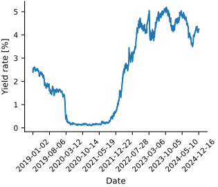
You can see how in March 2020 the yield rate dropped significantly due to the COVID-19 pandemic, and then it started to recover about 18 months later.

# Define Key dates
covid_start = '2020_03-12' # black thursday
recovery_start = '2021_09-12'

# Convert to datetime
covid_start = datetime.datetime.strptime(covid_start, "%Y_%m-%d")
recovery_start = datetime.datetime.strptime(recovery_start, "%Y_%m-%d")
recovery_start = (recovery_start - covid_start).days
date = pd.to_datetime(raw_date)
date = date - covid_start
date = date.dt.days
date = date.values

# Start data at the start of the pandemic
date_mask = date > 0
date = date[date_mask]
rate = rate[date_mask]

date = jnp.array(date, dtype=float)
rate = jnp.array(rate, dtype=float)

# Plot the data
plt.plot(date, rate, color='0.25', label='Two-year Treasury yield')
plt.axvline(recovery_start, color='black', linestyle='--', label='18 months after start of pandemic')
plt.axvline(x=1000, color='black', linestyle=':', label='1000 days after start of pandemic')
plt.xlabel("Calendar days since 12 March 2020")
plt.ylabel("Yield rate [%]")
plt.legend(loc='upper center', bbox_to_anchor=(0.5, -0.20), ncol=1)
finalize_axes(keep_box=False)
plt.show()

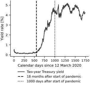
We take \(X_0\) to be the first observed yield on or after the recovery date and estimate \(\mu\) from observations at least 1,000 calendar days after the market crash. This is an illustrative calibration: we fit the mean curve and then estimate a variance scale. It is not a joint likelihood fit of the OU transition model.

recovery_index = int(jnp.argmax(date >= recovery_start))
x0 = rate[recovery_index]
late_mask = date >= 1000
mu = jnp.mean(rate[late_mask])

print(f'The initial yield is {x0:.4f}%')
print(f'The mean yield from calendar day 1000 onward is {mu:.4f}%')

# Time zero is the first observation used as X_0.
recovery_days = date[recovery_index:] - date[recovery_index]
recovery_rates = rate[recovery_index:]

The initial yield is 0.2100%
The mean yield from calendar day 1000 onward is 4.4743%

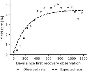
Now that we have established \(X_0\) and \(\mu\), we can fit the mean-reversion parameter \(\lambda\). The expectation of the process is

\[ \mathbb{E}[X_t] = X_0 e^{-\lambda t} + \mu (1 - e^{-\lambda t}) \]

We will just use a mean squared error loss function with a gradient descent optimizer to find the best \(\lambda\) fit the data.

def exp_X(x0, mu, theta, t):
    return x0 * jnp.exp(-theta * t) + mu * (1 - jnp.exp(-theta * t))

def compute_loss(lam, X, t, x0, mu):
    # Calculate the expected value of X_t based on the Ornstein-Uhlenbeck process
    X_expected = exp_X(x0, mu, lam, t)
    # Calculate the mean squared error between observed X and expected X
    return jnp.mean((X - X_expected) ** 2)

# Create a function to fit the mean reversion parameter
def find_lam(X, t, x0, mu, lam0=1.0, learning_rate=0.01, max_iters=5000, tol=1e-3):
    # Initialize lam
    lam = jnp.array(lam0)
    # Define the optimizer
    optimizer = optax.adam(learning_rate)
    opt_state = optimizer.init(lam)

    # Optimization loop
    def step(lam, opt_state):
        # Compute the gradient of the loss with respect to lam
        loss, grad_loss = jax.value_and_grad(compute_loss)(lam, X, t, x0, mu)
        # Apply optimizer step
        updates, opt_state = optimizer.update(grad_loss, opt_state)
        lam = optax.apply_updates(lam, updates)
        return lam, opt_state, loss

    # Iterative optimization
    loss_evolution = []
    for i in range(max_iters):
        lam, opt_state, loss = step(lam, opt_state)
        loss_evolution.append(loss)
        # Check for convergence
        if loss < tol:
            print(f"Converged in {i} iterations")
            break

    return float(lam), jnp.array(loss_evolution)

We fit on the dimensionless time \(\tau=t/T\), where \(T\) is the observed recovery horizon in days. The fitted rate is per unit \(\tau\); its value per day is \(\lambda/T\).

# Scaling the days to be between 0 and 1 for numerical stability
end_day = jnp.max(recovery_days)
s_days = recovery_days / end_day

# Fit the mean reversion parameter
lam, loss_evolution = find_lam(recovery_rates, s_days, x0, mu)

print(f"The estimated mean reversion parameter is {lam:.4}")

The estimated mean reversion parameter is 4.942

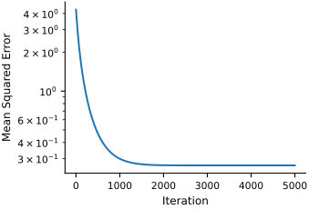
The loss history shows whether the mean-curve optimization has stabilized.

# Plot the loss evolution in log scale
plt.plot(loss_evolution)
plt.xlabel("Iteration")
plt.ylabel("Mean Squared Error")
plt.yscale('log')
finalize_axes(keep_box=False)
plt.show()

Compare the fitted mean curve with the observations.

# Plot the expected value of X_t based on the Ornstein-Uhlenbeck process
t = jnp.linspace(0, 1, 100)
X_expected = exp_X(x0, mu, lam, t)
plt.plot(recovery_days, recovery_rates, color='black', linestyle='none',
         marker='o', markerfacecolor='white', markeredgecolor='black',
         markersize=3, markevery=max(1, len(recovery_days) // 20),
         label='Observed rate')
plt.plot(t*end_day, X_expected, color='black', linestyle='--', linewidth=1.6,
         label='Expected rate')
plt.xlabel("Days since first recovery observation")
plt.ylabel("Yield rate [%]")
plt.legend(loc='upper center', bbox_to_anchor=(0.5, -0.20), ncol=2)
finalize_axes(keep_box=False)

array([<Axes: xlabel='Days since first recovery observation', ylabel='Yield rate [%]'>],
      dtype=object)

For deterministic \(X_0\), the OU variance at dimensionless time \(\tau\) is

\[ \operatorname{Var}[X_\tau]=\frac{\sigma^2}{2\lambda}(1-e^{-2\lambda\tau}). \]

We use the sample variance from calendar day 1,000 onward as a rough proxy for the terminal variance at \(\tau=1\), and solve this formula for \(\sigma\). Those observations are correlated and occur at different times, so this is a moment-based approximation, not an exact variance estimate. The daily diffusion amplitude is \(\sigma/\sqrt{T}\).

def estimate_sigma(var, lam, t):
    return jnp.sqrt(2 * lam * var / (-jnp.expm1(-2 * lam * t)))

assert lam > 0, "Mean reversion requires a positive fitted rate."
X_var = jnp.var(rate[late_mask], ddof=1)
sigma = estimate_sigma(X_var, lam, 1.0)
print(f"Volatility per square-root dimensionless time: {sigma:.4f}")
print(f"Mean reversion per day: {lam / end_day:.6f}")
print(f"Volatility per square-root day: {sigma / jnp.sqrt(end_day):.6f}")
# Check that the inferred amplitude reproduces the specified terminal variance.
assert bool(jnp.allclose(sigma**2 * (-jnp.expm1(-2 * lam)) / (2 * lam), X_var))

Volatility per square-root dimensionless time: 1.2582
Mean reversion per day: 0.004150
Volatility per square-root day: 0.036458

We simulate the process with the Euler–Maruyama scheme used for stochastic exponential growth. Only the drift term changes.

# Create a function to simulate the Ornstein-Uhlenbeck process
def ou_step(carry, dt):
    key, mu, lam, sigma, x = carry
    key, subkey = jr.split(key)
    # Compute the drift term
    drift = lam * (mu - x) * dt
    # Compute the diffusion term
    diffusion = sigma * jnp.sqrt(dt) * jr.normal(subkey)
    # Compute the new value of X
    x_new = x + drift + diffusion
    return (key, mu, lam, sigma, x_new), x_new

# Use 1,000 independent simulated paths
n_samples = 1000
# Initialize the random number generator
sim_keys = jr.split(jr.PRNGKey(0), n_samples)
dt = jnp.diff(t)

all_Xt = []

# Simulate the Ornstein-Uhlenbeck process
for i in range(n_samples):
    init_carry = (sim_keys[i], mu, lam, sigma, x0)
    _, X_simulated = jax.lax.scan(ou_step, init_carry, dt)
    Xt = jnp.concatenate((jnp.array([x0]), X_simulated))
    all_Xt.append(Xt)

all_Xt = jnp.array(all_Xt)

X_median = jnp.median(all_Xt, axis=0)
X_lower = jnp.quantile(all_Xt, 0.025, axis=0)
X_upper = jnp.quantile(all_Xt, 0.975, axis=0)

# Plot the expected value of X_t based on the Ornstein-Uhlenbeck process
plt.plot(recovery_days, recovery_rates, color='black', linestyle='none',
         marker='o', markerfacecolor='white', markeredgecolor='black',
         markersize=3, markevery=max(1, len(recovery_days) // 20),
         label='Observed rate')
plt.plot(t*end_day, X_median, color='black', linestyle='-', linewidth=1.7,
         label='Median rate')
plt.plot(t*end_day, X_expected, color='black', linestyle='--', linewidth=1.5,
         label='Expected rate')
plt.fill_between(t*end_day, X_lower, X_upper, facecolor='0.88',
                 edgecolor='0.55', hatch='///', linewidth=0.5, label='95% interval')
# Plot some samples
sample_styles = [':', '-.', (0, (5, 2))]
for i in range(3):
    plt.plot(t*end_day, all_Xt[i], color='0.45', linestyle=sample_styles[i],
             linewidth=0.8, label='Sample paths' if i == 0 else None)
plt.xlabel("Days since first recovery observation")
plt.ylabel("Yield rate [%]") 
plt.legend(loc='upper center', bbox_to_anchor=(0.5, -0.20), ncol=2)
finalize_axes(keep_box=False)
plt.show()

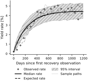
The simulated median can be compared with the analytic mean, and the pointwise interval with the observed yields. This checks the simulation and the scale of the illustrative fit; the same record was used for calibration, so it is not a held-out forecast test. A constant-parameter OU model cannot represent every change in the yield dynamics.

Vary the recovery date and late-data threshold, or fit the model to another series such as the 10-year Treasury note yield from the Federal Reserve Economic Data (FRED) database (Federal Reserve Bank of St. Louis, n.d.). An exact OU transition likelihood provides a way to estimate all parameters jointly.