

import matplotlib.pyplot as plt
%matplotlib inline
import matplotlib_inline
matplotlib_inline.backend_inline.set_matplotlib_formats('svg', 'pdf')
import seaborn as sns
Example: System Identification with Particle MCMC#
We again consider the system-identification problem, now using particle marginal Metropolis–Hastings to sample the parameter posterior. The particle filter supplies an unbiased estimate \(\widehat Z(\theta)=\widehat p(y_{1:T}\mid\theta)\) of the likelihood. The algorithm is:
Initialize \(\theta^{(0)}\)
Run a particle filter at \(\theta^{(0)}\) and compute \(\widehat Z(\theta^{(0)})\)
For \(k=1,\ldots,K\):
Propose a new parameter \(\theta' \sim q(\cdot \mid \theta^{(k-1)})\)
Run a new particle filter at \(\theta'\) and compute \(\widehat Z(\theta')\)
Compute the acceptance probability $\( a(\theta^{(k-1)},\theta') = \min\left(1, \frac{\widehat Z(\theta')p(\theta')q(\theta^{(k-1)} \mid \theta')}{\widehat Z(\theta^{(k-1)})p(\theta^{(k-1)})q(\theta' \mid \theta^{(k-1)})}\right) \)$
With probability \(a(\theta^{(k-1)},\theta')\), set \(\theta^{(k)}=\theta'\) and store \(\widehat Z(\theta')\); otherwise set \(\theta^{(k)}=\theta^{(k-1)}\) and keep the stored \(\widehat Z(\theta^{(k-1)})\)
import importlib.util
import json
import subprocess
import sys
from importlib import metadata

DAX_COMMIT = "084af6da51c95ea0807759022344c3cca07d0a64"
required_packages = {"diffrax": "diffrax", "optax": "optax", "blackjax": "blackjax", "seaborn": "seaborn"}
missing_packages = [package for module, package in required_packages.items() if importlib.util.find_spec(module) is None]
if missing_packages:
    subprocess.check_call([sys.executable, "-m", "pip", "install", *missing_packages])

try:
    direct_url = metadata.distribution("dax").read_text("direct_url.json")
    installed_dax_commit = json.loads(direct_url or "{}").get("vcs_info", {}).get("commit_id")
except metadata.PackageNotFoundError:
    installed_dax_commit = None

if installed_dax_commit != DAX_COMMIT:
    subprocess.check_call([
        sys.executable, "-m", "pip", "install", "--no-deps", "--force-reinstall",
        f"git+https://github.com/PredictiveScienceLab/dax.git@{DAX_COMMIT}",
    ])
import time
import equinox as eqx
import jax
import jax.random as jr
import jax.numpy as jnp
import dax

jax.config.update("jax_enable_x64", True)
key = jr.PRNGKey(0)
Duffing Oscillator#
We use the same stochastic Duffing dynamics and observation model as in the filtering, smoothing, and EM examples:
The Brownian motions and observation errors are independent. We keep \(\omega\), \(\gamma\), \(\sigma_x\), \(\sigma_v\), and the initial-state distribution (here \(\mathcal N(\boldsymbol 0,4I_2)\)) fixed and infer \(\theta=(\alpha,\beta,\delta,s)\). Thus \(s\) is the observation-noise standard deviation, not a process-diffusion parameter.
# Define the right-hand side, deterministic part of the Duffing oscillator
class DuffingControl(dax.ControlFunction):

    omega: jax.Array

    def __init__(self, omega):
        self.omega = jnp.array(omega)

    def _eval(self, t):
        # This is to avoid training the parameter
        omega = jax.lax.stop_gradient(self.omega)
        return jnp.cos(omega * t)


class Duffing(dax.StochasticDifferentialEquation):

    alpha: jax.Array
    beta: jax.Array
    delta: jax.Array

    gamma: jax.Array
    log_sigma_x: jax.Array
    log_sigma_v: jax.Array

    @property
    def sigma_x(self):
        return jnp.exp(self.log_sigma_x)

    @property
    def sigma_v(self):
        return jnp.exp(self.log_sigma_v)

    def __init__(self, alpha, beta, gamma, delta, sigma_x, sigma_v, u):
        super().__init__(control_function=u)
        self.alpha = jnp.array(alpha)
        self.beta = jnp.array(beta)
        self.delta = jnp.array(delta)

        self.gamma = jnp.array(gamma)
        self.log_sigma_x = jnp.log(sigma_x)
        self.log_sigma_v = jnp.log(sigma_v)

    def drift(self, x, u):
        # We won't train gamma
        gamma = jax.lax.stop_gradient(self.gamma)
        return jnp.array([x[1], -self.delta * x[1] - self.alpha * x[0] - self.beta * x[0] ** 3 + gamma * u])

    def diffusion(self, x, u):
        # We won't train sigma_x and sigma_v
        sigma_x = jax.lax.stop_gradient(self.sigma_x)
        sigma_v = jax.lax.stop_gradient(self.sigma_v)
        return jnp.array([sigma_x, sigma_v])
We will first define the true system parameters and generate our noisy data.
# True parameters
omega = 1.2
alpha = -1.0
beta = 1.0
delta = 0.3
gamma = 0.5
sigma_x = 0.01
sigma_v = 0.05
u = DuffingControl(omega)
true_sde = Duffing(alpha, beta, gamma, delta, sigma_x, sigma_v, u)

# True initial conditions
true_x0 = jnp.array([1.0, 0.0])

# Observation model
observation_function = dax.SingleStateSelector(0)
# Observation standard deviation
s = 0.1
true_likelihood = dax.GaussianLikelihood(s, observation_function)

# Generate synthetic data
t0 = 0.0
t1 = 40.0
dt = 0.1
key, path_key, observation_key = jr.split(key, 3)
sol = true_sde.sample_path(path_key, t0, t1, true_x0, dt=dt, dt0=0.05)
xs = sol.ys
ts = sol.ts
us = u(ts)
keys = jr.split(observation_key, xs.shape[0])
ys = true_likelihood.sample(xs, us, keys)

# Training data: transition n uses u(t_n) and is scored by y(t_{n+1}).
num_train_transitions = 200
us_train = us[:num_train_transitions]
ys_train = ys[1:num_train_transitions + 1]
We need a prior over the parameter coordinates and an observation likelihood. For continuity with the preceding example, we use an improper flat prior in \((\alpha,\beta,\delta,\log s)\); this choice is meaningful only when the resulting posterior is proper. Working with \(\log s\) keeps \(s\) positive.
# Prior
class SSMPrior(dax.Prior):

    def log_prob(self, theta):
        # Improper flat prior in alpha, beta, delta, and log(s).
        return 0.0

    def sample(self, key):
        return None

# Likelihood
class GaussianLikelihood(dax.Likelihood):

    log_s: jax.Array

    @property
    def s(self):
        return jnp.exp(self.log_s)

    def __init__(self, s):
        self.log_s = jnp.log(jnp.asarray(s))

    def _log_prob(self, y, x, u):
        return -0.5 * jnp.sum(((y - x[0]) / self.s) ** 2) - self.log_s

    def _sample(self, x, u, key):
        return x[0] + self.s * jr.normal(key)
Let’s initialize the parameters \(\theta^{(0)}\) for our chain to start from. Try adjusting the initial parameters and see how the chain behaves.
# Start a model from the wrong parameters
alpha_0 = -1.5
beta_0 = 1.5
delta_0 = 0.5
s_0 = 1.0

# The chain uses log(s), so this positive initial value is transformed below.
Construct a state-space model from each proposed parameter vector. Only the four entries of theta are proposed; the initial-state distribution and process-noise amplitudes remain fixed.
# Place the parameters in a dictionary
theta = {
    'alpha': alpha_0,
    'beta': beta_0,
    'delta': delta_0,
    'log_s': jnp.log(s_0),
}

# Create a state-space model from the parameters
def ssm_from_theta(theta):
    return dax.StateSpaceModel(
        dax.DiagonalGaussian(
            jnp.array([0.0, 0.0]),
            jnp.array([2.0, 2.0])),
        dax.EulerMaruyama(Duffing(theta['alpha'], theta['beta'], gamma, theta['delta'], sigma_x, sigma_v, u), dt=dt),
        GaussianLikelihood(jnp.exp(theta['log_s']))
    )
We are now set up to run particle MCMC. The particle count controls the noise in the likelihood estimate, while the proposal scale controls the acceptance and mixing of the parameter chain.
# Particle MCMC hyperparameters
num_particles = 1000
proposal_scale = 0.01
num_iters = 10000

prior = SSMPrior()
filter = dax.BootstrapFilter(num_particles=num_particles)
mcmc = dax.ParticleMCMC(prior, filter, proposal_scale, ssm_from_theta)

print('Running MCMC')

# Track the amount of time it takes to run the MCMC
mcmc_start = time.time()

final_state, (accept, log_Ls, thetas) = mcmc.run(theta, us_train, ys_train, num_iters, key)

mcmc_end = time.time()

print(f'MCMC took {mcmc_end - mcmc_start:.2f} seconds')
print(f'Acceptance rate: {jnp.mean(accept):.3f}')
Running MCMC
MCMC took 278.16 seconds
Acceptance rate: 0.215
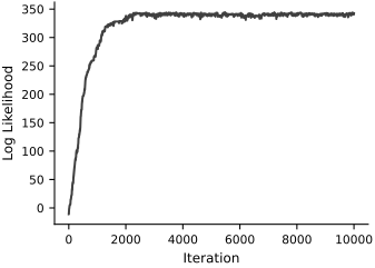
First inspect the estimated log-likelihood trace and the reported acceptance rate. These are useful debugging signals, but neither one establishes convergence of the parameter chain.
fig, ax = new_figure(size="half_standard")
ax.plot(log_Ls, color="0.25")
ax.set_xlabel('Iteration')
ax.set_ylabel('Log Likelihood')
finalize_axes(keep_box=False)
plt.show()
The parameter traces in Fig. 77 show how the chain moves through parameter space and can reveal sticking or slow exploration.
fig, ax = new_figure(size="full_tall", nrows=4, ncols=1, sharex=True)
trace_style = {"color": "0.35", "linewidth": 1.2}
truth_style = {"color": "black", "linestyle": "--", "linewidth": 1.1}

ax[0].plot(thetas['alpha'], label='PMCMC trace', **trace_style)
ax[0].axhline(alpha, label='Generating value', **truth_style)
ax[0].set_ylabel(r'$\alpha$')
ax[0].legend(loc='lower right', ncol=2)

ax[1].plot(thetas['beta'], **trace_style)
ax[1].axhline(beta, **truth_style)
ax[1].set_ylabel(r'$\beta$')

ax[2].plot(thetas['delta'], **trace_style)
ax[2].axhline(delta, **truth_style)
ax[2].set_ylabel(r'$\delta$')

ax[3].plot(jnp.exp(thetas['log_s']), **trace_style)
ax[3].axhline(s, **truth_style)
ax[3].set_xlabel('Iteration')
ax[3].set_ylabel(r'$s$')

finalize_axes(keep_box=False)
plt.show()
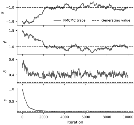
Fig. 77 Traces of the particle-MCMC chain for \(\alpha\), \(\beta\), \(\delta\), and \(s\) over 10,000 iterations. Dashed horizontal lines mark the generating values.#
The post-warmup marginal histograms are shown in Fig. 78. For this illustrative summary, discard the first 2,500 iterations as warmup and retain the remaining 7,500 draws. Before interpreting these histograms as posterior summaries, run multiple chains and report rank-normalized \(\widehat R\), bulk and tail effective sample sizes, and Monte Carlo standard errors.
# Do the histograms of the parameters
warmup = 2500
alpha_keep = thetas['alpha'][warmup:]
beta_keep = thetas['beta'][warmup:]
delta_keep = thetas['delta'][warmup:]
s_keep = jnp.exp(thetas['log_s'][warmup:])

fig, ax = new_figure(size="full_tall", nrows=4, ncols=1)
hist_style = {"bins": 20, "facecolor": "0.75", "edgecolor": "0.25", "linewidth": 0.5}
truth_style = {"color": "black", "linestyle": "--", "linewidth": 1.1}

ax[0].hist(alpha_keep, **hist_style)
ax[0].axvline(alpha, label='Generating value', **truth_style)
ax[0].set_xlabel(r'$\alpha$')
ax[0].set_ylabel('Frequency')
ax[0].legend(loc='upper right')

ax[1].hist(beta_keep, **hist_style)
ax[1].axvline(beta, **truth_style)
ax[1].set_xlabel(r'$\beta$')
ax[1].set_ylabel('Frequency')

ax[2].hist(delta_keep, **hist_style)
ax[2].axvline(delta, **truth_style)
ax[2].set_xlabel(r'$\delta$')
ax[2].set_ylabel('Frequency')

ax[3].hist(s_keep, **hist_style)
ax[3].axvline(s, **truth_style)
ax[3].set_xlabel(r'$s$')
ax[3].set_ylabel('Frequency')

finalize_axes(keep_box=False)
plt.show()
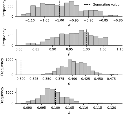
Fig. 78 Post-warmup marginal histograms for the 7,500 retained draws from the particle-MCMC run. Dashed vertical lines mark the generating parameter values.#
This short single-chain calculation is a computational demonstration, not a validated posterior analysis. Particle MCMC is substantially more expensive than the preceding EM point estimate because every proposal runs a particle filter, but it can represent parameter uncertainty once its Monte Carlo diagnostics are satisfactory. Experiment with the particle count and proposal scale, then run multiple chains before asking whether the apparent posterior concentration reflects practical identifiability.