Multifidelity Gaussian process surrogates

Multifidelity Gaussian process surrogates#

Example 1: Multi-fidelity regression of a synthetic function#

Suppose we have a high-fidelity model \(f_h\) and a low-fidelity model \(f_\ell\) of some phemonenon, given by

\[\begin{split} \begin{align*} f_h(x) &= \frac{1}{2} \sin\left( \frac{5}{2} x_1 + \frac{2}{3} x_2 \right)^2 + \frac{2}{3} e^{-x_1 (x_2 - \frac{1}{2})^2} \cos(4x_1 + x_2)^2 \\ f_\ell(x) &= 1.5 f_h(x) + \frac{1}{3} \sin(x_1 + x_2) + \frac{1}{2} e^{-x_1} \sin(x_1 + 7x_2). \end{align*} \end{split}\]

(These function definitions are modified from Perdikaris et al. (2015).)

We want to create a surrogate for \(f_h\).

Low-fidelity GP#

Suppose we have some low fidelity data \((\mathbf{X}_\ell, \mathbf{y}_\ell)\) and some high fidelity data \((\mathbf{X}_h, \mathbf{y}_h)\).

N_LOW_FIDELITY = 50
N_HIGH_FIDELITY = 8
N_TEST = 100

key, subkey = jr.split(key)
X_train_l, X_train_h, X_test, y_train_l, y_train_h, y_test_l, y_test_h = generate_synthetic_data(N_LOW_FIDELITY, N_HIGH_FIDELITY, N_TEST, key=subkey)

../../_images/5ac82bc28400cf31ad07e51d8dc91caa74190b92116bd8fe2d674f52de234bfc.svg

We’ll start by fitting a Gaussian process to the low fidelity data:

Show code cell source Hide code cell source

def build_gp(params, X):
    """Build a Gaussian process with RBF kernel.
    
    Parameters
    ----------
    params : dict
        Hyperparameters of the GP.
    X : ndarray
        Training data.
    
    Returns
    -------
    GaussianProcess
        The GP.
    """
    sigma = 1e-3  # Fixing the measurement noise
    amp = jnp.exp(params['log_amplitude'])
    ell = jnp.exp(params['log_lengthscales'])
    k = amp*transforms.Linear(1/ell, kernels.ExpSquared())  # Must be constructed this way if ell is a vector
    return GaussianProcess(k, X, diag=sigma**2)

def eval_gp(build_gp, Xq, X, y, params):
    """Evaluate a GP at query points Xq.
    
    Parameters
    ----------
    build_gp : callable
        A function that builds a GP from the hyperparameters.
    Xq : ndarray
        Query points.
    X, y: ndarray
        Training data.
    params : dict
        Hyperparameters of the GP.
    
    Returns
    -------
    GaussianProcess
        The conditioned GP.
    """
    gp = build_gp(params, X)
    _, cond_gp = gp.condition(y, Xq)
    return cond_gp

def loss(build_gp, params, X, y):
    """Negative marginal log likelihood of the GP."""
    gp = build_gp(params, X)
    return -gp.log_probability(y)

@eqx.filter_jit
def train_step_adam(carry, _, build_gp, X, y, optim, batch_size):
    params, opt_state, key = carry
    key, subkey = jr.split(key)
    idx = jr.randint(subkey, (batch_size,), 0, X.shape[0])
    value, grads = value_and_grad(partial(loss, build_gp))(params, X[idx], y[idx])
    updates, opt_state = optim.update(grads, opt_state)
    params = optax.apply_updates(params, updates)
    return (params, opt_state, key), value

def train_gp(build_gp, init_params, X, y, num_iters, learning_rate, batch_size, key):
    """Optimize the hyperparameters (xi) of a GP using the Adam optimizer.
    
    Parameters
    ----------
    init_params : dict
        Initial values of the hyperparameters.
    X, y: ndarray
        Training data.
    num_iters : int
        Number of optimization steps.
    learning_rate : float
        Learning rate for the optimizer.
    
    Returns
    -------
    dict
        The optimized hyperparameters.
    ndarray
        The loss values at each iteration.
    """
    
    # Initialize the optimizer
    optim = optax.adam(learning_rate)

    # Initialize the optimizer state
    init_carry = (init_params, optim.init(init_params), key)

    # Do optimization
    train_step = partial(train_step_adam, build_gp=build_gp, X=X, y=y, optim=optim, batch_size=batch_size)
    carry, losses = lax.scan(train_step, init_carry, None, num_iters)

    return carry[0], losses  # (optimized params, loss values)

params_l = {
    'log_amplitude': jnp.log(1.0),
    'log_lengthscales': jnp.log(jnp.array([1.0, 1.0]))
}

key, subkey = jr.split(key)
params_l, losses_l = train_gp(
    build_gp=build_gp, 
    init_params=params_l, 
    X=X_train_l, 
    y=y_train_l, 
    num_iters=5000, 
    learning_rate=1e-3,
    batch_size=10,
    key=subkey
)

Let’s visualize the low-fidelity data and the function \(f_\ell\).

X1, X2 = jnp.meshgrid(jnp.linspace(0, 1, 50), jnp.linspace(0, 1, 50))
Xq_plt = jnp.stack([X1.ravel(), X2.ravel()], axis=1)

cond_gp_plt = eval_gp(build_gp, Xq_plt, X_train_l, y_train_l, params_l)
Y_mean = cond_gp_plt.mean.reshape(*X1.shape)

../../_images/37d04513b211ef2a203ddcf1d276f39a78a42c5d5352e8a673dcb79f9ff06bd4.svg

Let’s check the fit of the low-fidelity GP to the low-fidelity data with a pairplot.

../../_images/b47fc4152a6264e182d0b5eee428e5726ab05b34fad44a9e546208cc57ab9d7b.svg

As expected, the low-fidelity GP matches the low-fidelity function \(f_\ell\) well, but it completely misses the high-fidelity function \(f_h\).

Multi-fidelity GP#

For the multi-fidelity GP, we’ll use the kernel

\[ k_h(x, x') = k\Big(\big(x, \tilde{m}_l(x)\big), \big(x', \tilde{m}_l(x')\big)\Big). \]

where \(\tilde{m}_l\) is the mean of the low-fidelity GP. In tinygp, this is best implemented with a tinygp.transforms.Transform object as below:

def generate_build_multi_fidelity_gp(build_gp, X_train_l, y_train_l, params_l):
    """Factory function for creating multi-fidelity GP builders."""

    def build_multi_fidelity_gp(params, X):
        """Build a multi-fidelity Gaussian process with RBF kernel."""
        sigma = 1e-3  # Fixing the measurement noise
        amp = jnp.exp(params['log_amplitude'])
        ell = jnp.exp(params['log_lengthscales'])
        ell_aug = jnp.exp(params['log_lengthscale_l'])  # Lengthscale for the low-fidelity GP mean

        # This is the mean, m_l, of the low-fidelity GP.
        # It is wrapped so that one simply needs to pass in a single input x vector.
        # It is also jitted.
        eval_low_fidelity_gp_mean = jit(lambda x: partial(eval_gp, build_gp)(x[None], X_train_l, y_train_l, params_l).mean)
        
        # This is the function that lifts the input x from e.g., 2 dimensions to 3 dimensions, 
        # where the 3rd dimension represents the low-fidelity GP mean.
        # It also applies the length scaling.
        lift_and_scale = lambda x: jnp.hstack([x/ell, eval_low_fidelity_gp_mean(x)/ell_aug])

        # The kernel is constructed in the lifted input space via a Transform.
        # The way Transform works is that for some transformation T, Transform(T, k1) produces
        # the kernel k(x, x') = k1(T(x), T(x')).
        k = amp*transforms.Transform(lift_and_scale, kernels.ExpSquared())

        return GaussianProcess(k, X, diag=sigma**2)
    
    return build_multi_fidelity_gp

Here’s how we can train the multi-fidelity GP:

params_m = {
    'log_amplitude': jnp.log(1.0),
    'log_lengthscales': jnp.log(jnp.array([1.0, 1.0])),
    'log_lengthscale_l': jnp.log(1.0)
}

build_multi_fidelity_gp = generate_build_multi_fidelity_gp(build_gp, X_train_l, y_train_l, params_l)

params_m, losses_m = train_gp(
    build_gp=build_multi_fidelity_gp,
    init_params=params_m, 
    X=X_train_h, 
    y=y_train_h, 
    num_iters=5000, 
    learning_rate=1e-3,
    batch_size=5,
    key=subkey
)

This is what the multi-fidelity GP looks like:

X1, X2 = jnp.meshgrid(jnp.linspace(0, 1, 50), jnp.linspace(0, 1, 50))
Xq_plt = jnp.stack([X1.ravel(), X2.ravel()], axis=1)

cond_gp_plt = eval_gp(build_multi_fidelity_gp, Xq_plt, X_train_h, y_train_h, params_m)
Y_mean = cond_gp_plt.mean.reshape(*X1.shape)

../../_images/73151a67d7a558b3b8161483e2adb9f9ae3b620326c02b04a65a981734377357.svg

Let’s compare the accuracy of the multi-fidelity GP to that of a GP fit only to the high fidelity data.

../../_images/0ff0a920e0700d62aa59ee4d2d8b467056541801d3f9e0f744d658e1d947457c.svg

The multi-fidelity GP has the most accurate predictions. Let’s visualize the mean predictive surface against the ground truth:

../../_images/caec24828a7eaf26b8bb5f56d0e308a9039fff671cb0c16db7c169310a7d4770.svg

The multi-fidelity GP \(\hat{f}_m\) approximates the high-fidelity model \(f_h\) fairly well! This is a significant improvement over naively fitting to the high-fidelity data alone.

Questions#

Decrease N_LOW_FIDELITY. How does the multi-fidelity GP \(\hat{f}_m\) perform with less low-fidelity data?
Decrease N_HIGH_FIDELITY. How does multi-fidelity GP \(\hat{f}_m\) perform with less high-fidelity data?
Increase N_HIGH_FIDELITY. At what point is the high-fidelity-only GP \(\hat{f}_h\) just as good as the multi-fidelity GP \(\hat{f}_m\)?
Add more terms (sin/cos, exponential, quadratic, or whetever you want) to low_fidelity_model. How different can the low-fidelity model \(f_\ell\) be from the high-fidelity model \(f_h\) and still get a good surrogate \(\hat{f}_m\)?

Example 2: Stochastic incompressible flow past a cylinder#

This example is taken from Perdikaris et al. (2015). Suppose you have a flow past a cylinder, subject to random inflow boundary conditions of the form

\[ U_\infty(x) = 1 + \sigma_1 \sin\left(\frac{\pi y}{9}\right) + \sigma_2 \left[\xi_1 \sin\left(\frac{\pi y}{9}\right) + \xi_2 \cos\left( \frac{\pi y}{9} \right) \right] \quad \xi_1, \xi_2 \sim \mathcal{N}(0, 1), \]

Let \(C_\text{BP}\) be the base pressure coefficient at the rear of the cylinder (see figure below, figure 9 from Perdikaris et al. (2015)).

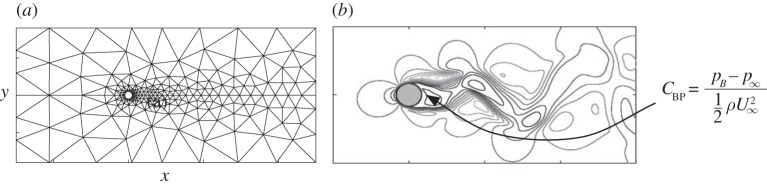
The quantity of interest is the mean of the upper 40% distribution for \(C_\text{BP}\), i.e. the superquantile risk \(f(x) \equiv \mathcal{R}_{0.6}[C_\text{BP}](x)\). We have two different-fidelity models that compute \(f\). To train the surrogate, we have 8 simulations from the high-fidelity model \(f_h\) and 99 simulations from the low-fidelity model \(f_\ell\).

Here are the data:

../../_images/b2140af20cba08b80d789a4cfdd7f96a02689855b6b9fbdbc1aca478362b85ee.svg

Multi-fidelity Gaussian process for superquantile risk#

As before, we first construct the low-fidelity GP surrogate:

params_l_cyl = {
    'log_amplitude': jnp.log(1.0),
    'log_lengthscales': jnp.log(jnp.array([1.0, 1.0]))
}

key, subkey = jr.split(key)
params_l_cyl, losses_l_cyl = train_gp(
    build_gp=build_gp, 
    init_params=params_l_cyl, 
    X=Xl_cyl, 
    y=yl_cyl, 
    num_iters=5000, 
    learning_rate=1e-3,
    batch_size=10,
    key=subkey
)

Next the multi-fidelity GP surrogate:

params_m_cyl = {
    'log_amplitude': jnp.log(1.0),
    'log_lengthscales': jnp.log(jnp.array([1.0, 1.0])),
    'log_lengthscale_l': jnp.log(1.0)
}

build_multi_fidelity_gp = generate_build_multi_fidelity_gp(build_gp, Xl_cyl, yl_cyl, params_l_cyl)

params_m_cyl, losses_m_cyl = train_gp(
    build_gp=build_multi_fidelity_gp,
    init_params=params_m_cyl, 
    X=Xh_cyl, 
    y=yh_cyl, 
    num_iters=5000, 
    learning_rate=1e-3,
    batch_size=5,
    key=subkey
)

And let’s also construct a surrogate on just the high-fidelity data, for comparison:

params_h_cyl = {
    'log_amplitude': jnp.log(1.0),
    'log_lengthscales': jnp.log(jnp.array([1.0, 1.0]))
}

key, subkey = jr.split(key)
params_h_cyl, losses_h_cyl = train_gp(
    build_gp=build_gp, 
    init_params=params_h_cyl, 
    X=Xh_cyl, 
    y=yh_cyl, 
    num_iters=5000, 
    learning_rate=1e-3,
    batch_size=10,
    key=subkey
)

As before, let’s visualize the predictive accuracy with some parity plots:

../../_images/2c4c846183c572ea1e0e626e4e4ac5193104bcb5f5487c412c49cf1e282a3491.svg

The multi-fidelity GP has the best predictive accuracy. Let’s visualize the response surface of the surrogate vs. the true high-fidelity model:

../../_images/9f473aea351901eaf963b62d712a3ff3a766901238aebff3255e7a7f080da1b3.svg

The surfaces are almost right on top of each other.