Sparsity-Promoting Regularization#
\(L^1\)-regularization is a method to prevent overfitting in linear models. It is also known as Lasso regression. It adds a penalty term to the loss function, which is the sum of the absolute values of the coefficients. This forces the coefficients to be small, and some of them to be exactly zero. This is useful for feature selection, as it allows us to discard some of the features.
Suppose we have \(N\) input–response pairs \((x_i,y_i)\) and \(M\) candidate features collected in \(\boldsymbol{\phi}(x)\). We fit the linear basis-function model:
Here \(\mathbf{w}\) contains the feature coefficients, \(w_0\) is the bias or intercept, and \(\epsilon\) is observation noise.
We can add the \(L^1\)-regularization term to the usual sum of square errors loss function:
where \(\lambda\geq0\) controls the penalty strength. The \(L^1\)-norm of the vector \(\mathbf{w}\) is defined as:
Notice that the bias term \(w_0\) is not regularized. We don’t want to push it to zero, as it is a constant term, and it is not related to the features.
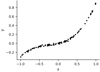
Let’s illustrate \(L^1\)-regularization with a simple example. We generate noisy data from a cubic polynomial and fit a larger library of polynomial and Fourier features. The penalty helps us select a smaller subset of terms.
Here are the data:
import numpy as np

rng = np.random.default_rng(697)
num_samples = 100
f = lambda x: 0.2 * x + 0.3 * x**2 + 0.4 * x**3
sigma = 0.01
x = rng.uniform(-1, 1, num_samples)
y = f(x) + rng.normal(0, sigma, num_samples)

fig, ax = plt.subplots(figsize=FIGURE_SIZES["half_standard"])
ax.plot(x, y, '.', color='k')
ax.set(xlabel='x', ylabel='y')
finalize_axes(keep_box=False)
array([<Axes: xlabel='x', ylabel='y'>], dtype=object)
We will try to fit a ridiculously complicated model. We will have a degree-ten polynomial, and then we will also add a bunch of Fourier terms:
from jax import config
config.update("jax_enable_x64", True)
import jax.numpy as jnp
from jax import vmap

@vmap
def features(x):
    tmp1 = jnp.array([x ** i for i in range(1, 11)])
    tmp2 = jnp.array([jnp.sin(2 * np.pi * x * i) for i in range(1, 11)])
    return jnp.concatenate([tmp1, tmp2])
Visualize the features:
xs = jnp.linspace(-1, 1, 200)
Phi = features(xs)
fig, ax = plt.subplots(figsize=FIGURE_SIZES["half_standard"])
ax.plot(xs, Phi, lw=0.2)
ax.set(xlabel='x', ylabel='feature value')
finalize_axes(keep_box=False)
array([<Axes: xlabel='x', ylabel='feature value'>], dtype=object)
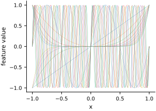
Clearly an overkill. But Lasso regression will still be able to throw away the unnecessary terms.
In what follows we do Lasso regression using the sklearn library.
We use LassoCV, which also does cross-validation to find the best value of the regularization parameter \(\lambda\).
from sklearn import linear_model

Phi_train = features(x)
clf = linear_model.LassoCV(fit_intercept=True, max_iter=100000, tol=1e-8)
clf.fit(Phi_train, y)
lr = linear_model.RidgeCV(fit_intercept=True)
lr.fit(Phi_train, y)
The library contains ten nonconstant monomials and ten sine terms. Both fits estimate a separate, unpenalized intercept, which is excluded from the coefficient panels. Scikit-learn uses a factor \(1/(2N)\) for the Lasso squared-error term, so its parameter \(\alpha\) corresponds to \(\lambda/2\) in our convention.
For comparison, we do Ridge regression (which adds an L2-regularization term) also with cross-validation.
fig, axes = plt.subplots(2, 1, figsize=(7.35, 2.2))
axes[0].imshow(clf.coef_.reshape(1, 20), cmap='gray', vmin=-0.5, vmax=0.5)
axes[0].set(xlabel='feature index', title='Lasso',
            xticks=np.arange(0, 20, 2), xticklabels=np.arange(0, 20, 2),
            yticks=[])
axes[1].imshow(lr.coef_.reshape(1, 20), cmap='gray', vmin=-0.5, vmax=0.5)
axes[1].set(xlabel='feature index', title='Ridge',
            xticks=np.arange(0, 20, 2), xticklabels=np.arange(0, 20, 2),
            yticks=[])
finalize_axes(keep_box=True)
array([<Axes: title={'center': 'Lasso'}, xlabel='feature index'>,
       <Axes: title={'center': 'Ridge'}, xlabel='feature index'>],
      dtype=object)
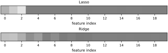
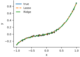
We see that Ridge regression has a lot more non-zero coefficients than Lasso regression.
Let’s visualize the predictions as well:
Phi_test = features(xs)
lass_pred = clf.predict(Phi_test)
ridge_pred = lr.predict(Phi_test)

fig, ax = plt.subplots(figsize=FIGURE_SIZES["half_standard"])
ax.plot(x, y, '.', color='k')
ax.plot(xs, f(xs), lw=2, label='true')
ax.plot(xs, lass_pred, '--', lw=2, label='Lasso')
ax.plot(xs, ridge_pred, '-.', lw=2, label='Ridge')
ax.set(xlabel='x', ylabel='y')
ax.legend(loc='best')
finalize_axes(keep_box=False)
array([<Axes: xlabel='x', ylabel='y'>], dtype=object)
Geometry of the \(L^1\) penalty#
To understand how Lasso regression works, we need to look at the \(L^1\)-norm. Let’s work with just two parameters: \(\mathbf{w} = (w_1,w_2)\). The \(L^1\)-norm is:
This is also called the Manhattan norm. The name reflects the distance traveled along the grid of city blocks.
Let’s consider a simple quadratic objective function:
where \(\mathbf{A}\) is symmetric positive definite, so the minimum is at \(\mathbf{w}^*\). We seek the minimum of the \(L^1\)-regularized objective function
To understand this minimum, first we need to mention that Lasso regression is equivalent to the following constrained optimization problem:
To see that this is equivalent to the \(L^1\)-regularized problem, we can use the Lagrange multiplier method. For a penalized minimizer \(\widehat{\mathbf{w}}_\lambda\), setting \(t=\|\widehat{\mathbf{w}}_\lambda\|_1\) gives the same constrained minimizer. Conversely, a Lagrange multiplier supplies a corresponding penalty for a positive constraint radius. This correspondence need not be one-to-one: several penalties can give the zero solution, and sufficiently large radii leave the unpenalized solution unchanged.
Now, we can understand what is going on by looking at the level sets of \(f(\mathbf{w})\) and \(\|\mathbf{w}\|_1\).
array([<Axes: xlabel='$w_1$', ylabel='$w_2$'>], dtype=object)
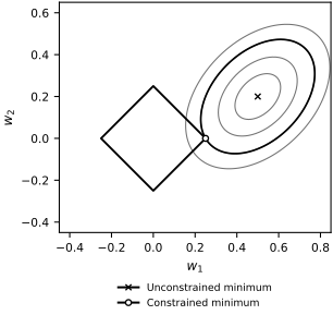
For the plotted radius \(t=0.25\), the constrained minimum is \((0.25,0)\), where the quadratic contour touches a corner of the diamond. You are trying to get to the minimum of \(f(\mathbf{w})\) while remaining inside the diamond \(\|\mathbf{w}\|_1 \leq t\). The level sets of \(\|\mathbf{w}\|_1\) are diamonds. The constrained minimum of \(f(\mathbf{w})\) will be where a level set of \(f(\mathbf{w})\) first touches the diamond. You will often find yourself at a corner of the diamond. Then one of the components of \(\mathbf{w}\) will be zero.
Bayesian Interpretation of Lasso Regression#
Lasso regression can be interpreted as a Bayesian method. To see this, put a Laplace prior on each one of the weights:
The density of the Laplace distribution is:
Taking the logarithm of the Laplace prior, we get:
Therefore, we see that (assuming a Gaussian likelihood), the \(L^1\)-regularized objective function is (up to an additive constant) equal to the negative log posterior.
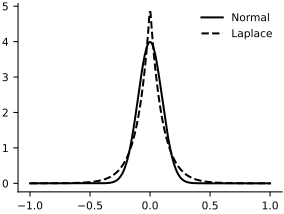
Let’s visualize the Laplace and Gaussian densities:
import scipy.stats as st

xs = np.linspace(-1, 1, 300)
fig, ax = plt.subplots(figsize=FIGURE_SIZES["half_standard"])
ax.plot(xs, st.norm.pdf(xs, 0, 0.1), color='black', linestyle='-',
        label='Normal')
ax.plot(xs, st.laplace.pdf(xs, 0, 0.1), color='black', linestyle='--',
        label='Laplace')
ax.legend()
finalize_axes(keep_box=False)
array([<Axes: >], dtype=object)