import matplotlib.pyplot as plt
%matplotlib inline
import matplotlib_inline
matplotlib_inline.backend_inline.set_matplotlib_formats('svg')
import seaborn as sns

import jax
from jax import grad, vmap, jit
import jax.numpy as jnp
import jax.scipy.stats as jst
import optax

jax.config.update("jax_enable_x64", True)

The Laplace Approximation

The Laplace approximation is a method to approximate a probability distribution with a Gaussian distribution. The method is based on the Taylor expansion of the logarithm of the probability distribution around the mode of the distribution. The Laplace approximation is a useful tool in Bayesian statistics, where it is used to approximate the posterior distribution of a parameter given some data.

The Taylor Expansion in Higher Dimensions

Let \(g:\mathbb{R}^d\rightarrow \mathbb{R}\) and \(x_0\in\mathbb{R}^d\). The Taylor series expansion is:

\[\begin{split} \begin{aligned} g(x) ={}& g(x_0) + \sum_{i=1}^d\frac{\partial g}{\partial x_i}(x_0)(x_i-x_{0i}) \\ &+\frac{1}{2}\sum_{i,j=1}^d\frac{\partial^2g}{\partial x_i\partial x_j}(x_0)(x_i-x_{0i})(x_j-x_{0j}) + \dots. \end{aligned} \end{split}\]

Another way of writing this is:

\[\begin{split} \begin{aligned} g(x) ={}& g(x_0) + \nabla g(x_0)^T(x-x_0) \\ &+ \frac{1}{2}(x-x_0)^T\nabla^2 g(x_0) (x-x_0) + \dots, \end{aligned} \end{split}\]

where the gradient is the column vector

\[ \nabla g(x_0) = \left(\frac{\partial g}{\partial x_1}(x_0),\dots,\frac{\partial g}{\partial x_d}(x_0)\right)^T, \]

and the Hessian is:

\[ \nabla^2 g(x_0) = \left(\frac{\partial^2g}{\partial x_i\partial x_j}(x_0)\right)_{i,j=1}^d. \]

The Laplace Approximation in 1D

Near an isolated interior mode, if the log density is twice differentiable and has a negative-definite Hessian, the density can be approximated locally by a Gaussian. This approximation may be poor for skewed, heavy-tailed, multimodal, bounded, or weakly identified distributions (Tierney and Kadane, 1986). Consider a probability density \(p(x)\) on the real line. Assume that \(p(x)>0\) in a neighborhood of the mode, so we can work with its logarithm. First, we find the maximum of \(\log p(x)\), which is called the mode (or just the maximum):

\[ x_0 = \arg\max_x \log p(x). \]

Then, we take the Taylor expansion of \(\log p(x)\) about \(x=x_0\):

\[ \log p(x) = \log p(x_0) + (\log p)'(x_0) (x-x_0) + \frac{1}{2}(\log p)''(x_0) (x-x_0)^2 + \dots. \]

Since \(x_0\) is a critical point of \(\log p(x)\), we must have that:

\[ (\log p)'(x_0) = 0. \]

So, the expansion becomes:

\[ \log p(x) \approx \frac{1}{2}(\log p)''(x_0) (x-x_0)^2 + \text{const}. \]

Therefore,

\[ p(x) \propto \exp\left\{ \frac{1}{2}(\log p)''(x_0) (x-x_0)^2 \right\}. \]

Under the nondegeneracy assumption above, \((\log p)''(x_0)<0\). Therefore, the number:

\[ c^2 = -\left[(\log p)''(x_0)\right]^{-1}, \]

is positive. By inspection then, we see that:

\[ p(x) \propto \exp\left\{-\frac{(x-x_0)^2}{2c^2}\right\}. \]

Ignoring all higher order terms, we conclude:

\[ p(x) \approx \mathcal{N}\left(x|x_0, -\left[(\log p)''(x_0)\right]^{-1}\right). \]

This is the Laplace approximation in one dimension.

Example: Gamma Distribution

Let’s try it out with the gamma distribution. First I am going to write a quick function to help us minimize the negative log likelihood of the gamma distribution.

# Optimization function using Optax (for scalar minimization)
def find_minimum(fun, init_x, max_iter=5000, tol=1e-6):
    optimizer = optax.adam(learning_rate=0.01)
    opt_state = optimizer.init(init_x)
    
    def step(x, opt_state):
        loss, grad_val = jax.value_and_grad(fun)(x)
        updates, opt_state = optimizer.update(grad_val, opt_state, x)
        x = optax.apply_updates(x, updates)
        return x, opt_state, loss

    x = init_x
    for _ in range(max_iter):
        x, opt_state, loss = step(x, opt_state)
        if jnp.abs(grad(fun)(x)) < tol:
            status = 'converged'
            break
        
    status = 'maximum iterations reached'

    return x, loss, status

We first formulate the minimization problem. Maximizing the probability density is equivalent to minimizing its negative logarithm.

# Construct the -log pdf of a gamma distribution
alpha = 10
minus_log_pdf_true = lambda x: -jst.gamma.logpdf(x, alpha)

# Find the maximum using an optimization method 
init_x = 1.0
x_0, min_logpdf_val, status = find_minimum(minus_log_pdf_true, init_x)

# Return the maximum of the pdf
p_0 = jnp.exp(-min_logpdf_val)

print(f'The maximum of the gamma pdf is {p_0:.4f} at x = {x_0:.4f}.')

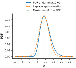
The maximum of the gamma pdf is 0.1318 at x = 8.9997.

We can prove this to ourselves by checking the derivative of the negative log likelihood of the gamma distribution. It should be zero at the maximum.

dp_0 = grad(minus_log_pdf_true)(x_0)
print(f'The derivative of the log pdf at the maximum is: {dp_0:.4f}.')

The derivative of the log pdf at the maximum is: -0.0000.

Great. We can trust that we found the maximum. We need one more thing for the Laplace approximation: the standard deviation of our Gaussian. To get this, we need to calculate the second derivative of the log likelihood of the gamma distribution.

# Compute the second derivative of the log pdf at the maximum
d2p_0 = grad(grad(minus_log_pdf_true))(x_0)
std = jnp.sqrt(1. / d2p_0)

# Define the range of x values to plot
x = jnp.linspace(x_0 - 6 * std, x_0 + 6 * std, 200)

# Build the Gaussian approximation to the gamma pdf
approx = lambda d: jst.norm.pdf(x, loc=x_0, scale=std)

See how painless this all was with the power of JAX? Let’s plot both distributions to verify our approximation.

# Plot the results
fig, ax = plt.subplots(figsize=FIGURE_SIZES["half_standard"])
pdf_true = jst.gamma.pdf(x, alpha)
ax.plot(x, pdf_true, label='PDF of Gamma(%.2f)' % alpha)
ax.plot(x, approx(x), '--', label='Laplace approximation')
ax.plot([x_0] * 10, jnp.linspace(0, p_0, 10), ':', label='Maximum of true PDF')
ax.legend(
    loc="lower center", bbox_to_anchor=(0.5, 1.02),
    ncol=1, borderaxespad=0.0,
)
ax.set_xlabel('$x$')
ax.set_ylabel('PDF')
finalize_axes(keep_box=False)
plt.show()

The Laplace Approximation in Many Dimensions

As in one dimension, let \(x_0=\arg\max_x\log p(x)\) and take the Taylor expansion of \(\log p(x)\) about \(x=x_0\):

\[\begin{split} \begin{aligned} \log p(x) ={}& \log p(x_0) + \nabla \log p(x_0)^T (x-x_0) \\ &+ \frac{1}{2}(x-x_0)^T\nabla^2 \log p(x_0) (x-x_0) + \dots. \end{aligned} \end{split}\]

Since \(x_0\) is a critical point of \(\log p(x)\), we must have that:

\[ \nabla \log p(x_0) = 0. \]

So, the expansion becomes:

\[ \log p(x) \approx \frac{1}{2}(x-x_0)^T\nabla^2 \log p(x_0) (x-x_0) + \text{const}. \]

Therefore,

\[ p(x) \propto \exp\left\{ \frac{1}{2}(x-x_0)^T\nabla^2 \log p(x_0) (x-x_0) \right\}. \]

Assume that the Hessian \(\nabla^2 \log p(x_0)\) is negative definite. Therefore, the matrix:

\[ C = -(\nabla^2\log p(x_0))^{-1}, \]

is positive definite. By inspection then, we see that:

\[ p(x) \propto \exp\left\{-\frac{1}{2}(x-x_0)^TC^{-1}(x-x_0)\right\}. \]

Ignoring all higher order terms, we conclude:

\[ p(x) \approx \mathcal{N}\left(x|x_0, -(\nabla^2\log p(x_0))^{-1}\right). \]

This is the Laplace approximation in many dimensions.

The Laplace Approximation of the Posterior

If you have a linear model and a Gaussian likelihood and the prior \(p(x)\) is Gaussian, then the posterior \(p(x|y)\) is Gaussian. In general, you can only characterize the posterior through sampling or some approximation. Sampling from the posterior is developed later in the Sampling from Posteriors section. For now, let us discuss the Laplace approximation to the posterior.

The Laplace approximation finds a Gaussian approximation to the posterior. For simplicity we will work with a Gaussian likelihood, but these ideas can be applied to any likelihood. To avoid over complicating things on this first attempt, let us assume that we know the value of \(\sigma\). We will generalize our approach later. Our posterior (for just \(x\)) is:

\[\begin{split} \begin{aligned} p(x|y,\sigma) &\propto p(y|x,\sigma)p(x) \\ &= \mathcal{N}\left(y|f(x),\sigma^2 I\right)p(x) \\ &\propto \exp\left\{-\frac{\lVert y - f(x) \rVert_2^2}{2\sigma^2}\right\}p(x). \end{aligned} \end{split}\]

To implement the Laplace approximation define:

\[ L(x) = -\frac{\lVert y - f(x) \rVert_2^2}{2\sigma^2} + \log p(x). \]

We need to find the maximum of this:

\[ \mu = \arg\max_{x\in\mathcal{X}} L(x), \]

the matrix

\[ \Sigma = -\left(\nabla^2 L(\mu)\right)^{-1}, \]

and the approximation is:

\[ p(x|y,\sigma) \approx \mathcal{N}(x|\mu,\Sigma). \]

The second derivative is:

\[\begin{split} \begin{aligned} \frac{\partial ^2 L}{\partial x_j \partial x_r}(\mu) &= -\frac{1}{\sigma^2}\sum_{i=1}^m\frac{\partial f_i}{\partial x_j}(\mu)\frac{\partial f_i}{\partial x_r}(\mu) \\ &\quad+\frac{1}{\sigma^2}\sum_{i=1}^m(y_i-f_i(\mu))\frac{\partial^2 f_i}{\partial x_j\partial x_r}(\mu) \\ &\quad+ \frac{\partial^2\log p}{\partial x_j\partial x_r}(\mu). \end{aligned} \end{split}\]

Thus, the Laplace approximation requires second derivatives of the model.