Structural Identifiability of a Harmonic Oscillator#

Consider the undamped harmonic oscillator

\[ m\ddot{x}(t)=-kx(t), \qquad x(0)=x_0, \qquad \dot{x}(0)=v_0, \]

where \(m>0\) is the mass, \(k>0\) is the spring constant, and the initial state \((x_0,v_0)\) is known. Its position is

\[ x(t;m,k)=x_0\cos(\omega t)+\frac{v_0}{\omega}\sin(\omega t), \qquad \omega^2=\frac{k}{m}. \]

The complete position trajectory therefore depends on \(m\) and \(k\) only through the ratio \(k/m\). The parameter-to-observable map is unchanged along every admissible curve \(k=\omega^2m\), so position data cannot identify \(m\) and \(k\) separately. This is structural nonidentifiability: it follows from the parameter-to-observable map itself, before a data set or inference algorithm is chosen (Raue et al., 2009).

Statistical model#

We observe position at times \(t_1,\ldots,t_N\) and use the model

\[ y_i=x(t_i;m,k)+\epsilon_i, \qquad \epsilon_i\mathrel{\overset{\mathrm{iid}}{\sim}}\operatorname{Normal}(0,\sigma^2). \]

The unknown vector is \(\theta=(m,k,\sigma)\), while the initial state is fixed at \(x_0=1\) and \(v_0=0\). We assign independent priors

\[ m\sim\operatorname{Uniform}(1,2), \quad k\sim\operatorname{Uniform}(0.5,3), \quad \log\sigma\sim\operatorname{Normal}(-3,0.5^2). \]

These proper priors produce a proper posterior, but they do not restore information that is absent from the likelihood: the posterior for \((m,k)\) retains a ridge along nearly constant \(k/m\) (Stuart, 2010). The computation below illustrates this geometry.

# Containers for storing parameters
class OscillatorState(NamedTuple):
    x: float
    v: float

class OscillatorParams(NamedTuple):
    m: float
    k: float
    init_cond: OscillatorState

class MeasurementParams(NamedTuple):
    sigma: float

class Params(NamedTuple):
    oscillator: OscillatorParams
    measurement: MeasurementParams

Unconstrained coordinates#

NUTS operates most conveniently in unconstrained coordinates. We therefore define an invertible map \(T:\mathbb{R}^3\rightarrow\Theta\) and write \(\theta=T(\xi)\), where \(\Theta=(1,2)\times(0.5,3)\times(0,\infty)\) and

\[ \xi_j\mathrel{\overset{\mathrm{iid}}{\sim}}\operatorname{Normal}(0,1), \qquad j=1,2,3. \]

Gaussian cumulative-distribution transforms of \(\xi_m=\xi_1\) and \(\xi_k=\xi_2\) generate the uniform priors for \(m\) and \(k\), while \(\sigma=\exp(-3+0.5\xi_\sigma)\) with \(\xi_\sigma=\xi_3\) generates the lognormal prior.

Hide code cell source

def normal_to_uniform(x, a, b):
    """Transforms from N(0, 1) to U(a, b)."""
    return dist.Normal().cdf(x)*(b - a) + a

def uniform_to_normal(x, a, b):
    """Transforms from U(a, b) to N(0, 1)."""
    return dist.Normal().icdf((x - a)/(b - a))

def exp_transform(x, shift, scale):
    return jnp.exp(x*scale + shift)

def log_transform(x, shift, scale):
    return (jnp.log(x) - shift)/scale

class ParamsTransformation:
    def __init__(self, m_low, m_high, k_low, k_high, sigma_shift, sigma_scale, init_cond=None):
        self.m_low = m_low
        self.m_high = m_high
        self.k_low = k_low
        self.k_high = k_high
        self.sigma_shift = sigma_shift
        self.sigma_scale = sigma_scale
        self.init_cond = init_cond if init_cond is not None else OscillatorState(x=None, v=None)
        self.split_xi_fn = None
        params_tmp = Params(
            oscillator=OscillatorParams(
                m=0.5*(m_low + m_high),
                k=0.5*(k_low + k_high),
                init_cond=self.init_cond,
            ),
            measurement=MeasurementParams(sigma=jnp.exp(sigma_shift)),
        )
        xi_tmp = self.backward(params_tmp)  # This is just to set unflatten and split functions
        self._n_params = xi_tmp.shape[0]

    def forward(self, xi: ArrayLike) -> Params:
        """Maps from unconstrained to constrained space."""
        osc_, meas_ = self.split_xi_fn(xi)

        # ODE model parameters
        m = normal_to_uniform(osc_[0], self.m_low, self.m_high)
        k = normal_to_uniform(osc_[1], self.k_low, self.k_high)
        osc = OscillatorParams(m=m, k=k, init_cond=self.init_cond)

        # Measurement model parameters
        sigma = exp_transform(meas_[0], self.sigma_shift, self.sigma_scale)
        meas = MeasurementParams(sigma=sigma)

        return Params(oscillator=osc, measurement=meas)
    
    def backward(self, p: Params) -> Array:
        """Maps from constrained to unconstrained space."""
        # ODE model parameters
        xi_m = uniform_to_normal(p.oscillator.m, self.m_low, self.m_high)
        xi_k = uniform_to_normal(p.oscillator.k, self.k_low, self.k_high)
        xi_osc = jnp.hstack((xi_m, xi_k))
        
        # Measurement model parameters
        xi_sigma = log_transform(p.measurement.sigma, self.sigma_shift, self.sigma_scale)
        xi_meas = jnp.hstack((xi_sigma,))
        
        # Combine
        xi, f = ravel_pytree((xi_osc, xi_meas))
        if self.split_xi_fn is None:
            self.split_xi_fn = f
        
        return xi
    
    @property
    def n_params(self):
        return self._n_params
T = ParamsTransformation(
    m_low=1.0,
    m_high=2.0,
    k_low=0.5,
    k_high=3.0,
    sigma_shift=-3,
    sigma_scale=0.5,
    init_cond=OscillatorState(x=1.0, v=0.0)
)
Hide code cell source

xi_samples = dist.Normal().sample(key, (10000, T.n_params))
theta_samples = vmap(T.forward)(xi_samples)

fig, ax = plt.subplots(1, 3, figsize=FIGURE_SIZES["full_landscape"], constrained_layout=True)
for i, name in enumerate([r"$\xi_1$", r"$\xi_2$", r"$\xi_3$"]):
    ax[i].hist(xi_samples[:, i], bins=20, density=True, color="0.75", edgecolor="black")
    ax[i].set_xlabel(name)
    ax[i].set_yticks([])
finalize_axes(keep_box=False);

fig, ax = plt.subplots(1, 3, figsize=FIGURE_SIZES["full_landscape"], constrained_layout=True)
ax[0].hist(theta_samples.oscillator.m, bins=20, density=True, color="0.75", edgecolor="black")
ax[1].hist(theta_samples.oscillator.k, bins=20, density=True, color="0.75", edgecolor="black")
ax[2].hist(theta_samples.measurement.sigma, bins=20, density=True, color="0.75", edgecolor="black")
for i, name in enumerate([r"$m$", r"$k$", r"$\sigma$"]):
    ax[i].set_xlabel(name)
    ax[i].set_yticks([])
finalize_axes(keep_box=False);
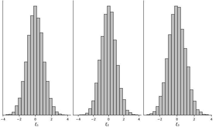
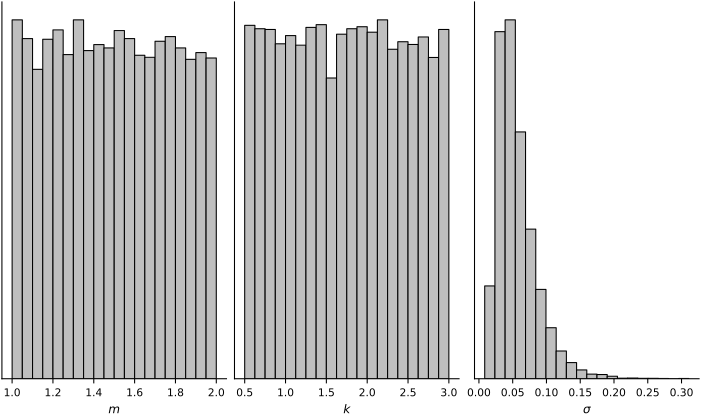
Prior histograms in unconstrained coordinates and after transformation to mass, stiffness, and noise scale. Prior histograms in unconstrained coordinates and after transformation to mass, stiffness, and noise scale.

The transformed samples recover the intended priors in physical coordinates. The following class collects the prior, likelihood, and predictive distributions.

Hide code cell source

class ProbabilisticDynamicalSystem:
    """Probabilistic model for a dynamical system."""

    def __init__(self, params_transform, solver):
        """Initialize the model.

        Parameters
        ----------
        params_transform: ParamsTransformation
            An invertible mapping between xi (unconstrained space) and theta (constrained space).
        solver: Callable
            A function that takes a time vector and a set of parameters and returns the state of the system.
        """
        self.params_transform = params_transform
        self.solver = solver
    
    def __call__(self, t, xi, *, key):
        return self.sample_predictive(t, xi, key=key)
    
    def log_prior(self, xi):
        """Prior log density."""
        return jnp.sum(dist.Normal().log_prob(xi))
    
    def log_likelihood(self, xi, obs_times, obs_positions):
        """Likelihood log density."""
        params = self.params_transform.forward(xi)
        positions = self.solver(obs_times, params.oscillator).x
        return jnp.sum(dist.Normal(positions, params.measurement.sigma).log_prob(obs_positions))
    
    def log_posterior(self, xi, obs_times, obs_positions):
        """Posterior log density."""
        return self.log_prior(xi) + self.log_likelihood(xi, obs_times, obs_positions)

    def sample_prior(self, *, key, num_samples=None):
        """Sample xi."""
        return dist.Normal().rsample(key, sample_shape=self._get_sample_shape(num_samples))

    def sample_predictive(self, t, xi, *, key, num_samples=None):
        """Sample from the predictive distribution (given xi) at times t."""
        params = self.params_transform.forward(xi)
        x = self.solver(t, params.oscillator).x
        return dist.Normal(x, params.measurement.sigma).rsample(key)

    def sample_prior_predictive(self, t, *, key, num_samples=None):
        """Sample from the prior predictive distribution at times t."""
        key_xi, key_y = jrandom.split(key)
        if num_samples is None:
            xi = self.sample_prior(key_xi)
            return self.sample_predictive(t, xi, key=key_y)
        else:
            sample_prior_vmapped = vmap(lambda k: self.sample_prior(key=k))
            sample_predictive_vmapped = vmap(lambda t, xi, k: self.sample_predictive(t, xi, key=k), in_axes=(None, 0, 0))
            xi = sample_prior_vmapped(jrandom.split(key_xi, num_samples))
            return sample_predictive_vmapped(t, xi, jrandom.split(key_y, num_samples))
    
    def _get_sample_shape(self, num_samples=None):
        d = self.params_transform.n_params
        return (num_samples, d) if num_samples is not None else (d,)

def harmonic_oscillator(
    t: ArrayLike, 
    params: OscillatorParams
) -> OscillatorState:
    """Analytic solution to the harmonic oscillator ODE system."""
    m = params.m
    k = params.k
    init = params.init_cond
    omega = (k/m)**0.5
    position = init.x*jnp.cos(omega*t) + init.v/omega*jnp.sin(omega*t)
    velocity = -init.x*omega*jnp.sin(omega*t) + init.v*jnp.cos(omega*t)
    return OscillatorState(x=position, v=velocity)
prob_model = ProbabilisticDynamicalSystem(T, harmonic_oscillator)

Prior predictive trajectories#

Prior predictive trajectories show the range of motions allowed before observing data.

# 1. Sample the prior for xi (this is just a standard Gaussian)
key, subkey = jrandom.split(key)
_xi_prior_samples = prob_model.sample_prior(key=subkey, num_samples=300)

# 2. Transform xi (unconstrained) to theta (constrained)
_theta_prior_samples = vmap(T.forward)(_xi_prior_samples)

# 3. Solve the ODE system for each theta sample
times_plt = jnp.linspace(0, 10, 200)
x_plt = vmap(harmonic_oscillator, in_axes=(None, 0))(times_plt, _theta_prior_samples.oscillator).x

# 4. Plot the samples
fig, ax = plt.subplots(figsize=FIGURE_SIZES["half_standard"], constrained_layout=True)
ax.plot(times_plt, x_plt.T, lw=0.7, alpha=0.12, color="0.25", rasterized=True)
ax.set_xlabel("Time")
ax.set_ylabel("Position")
finalize_axes(keep_box=False);
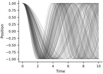
Prior-predictive oscillator position trajectories over time.

Synthetic observations#

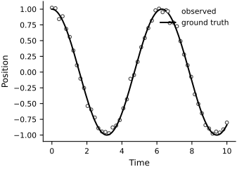
We generate observations at \(50\) equally spaced times from \(m=1.5\), \(k=1.5\), and \(\sigma=0.05\). The true ratio is therefore \(\omega^2=k/m=1\).
Hide code cell source

# Create a ground truth
init_cond = OscillatorState(x=1.0, v=0.0)
ground_truth_params = Params(
    oscillator=OscillatorParams(m=1.5, k=1.5, init_cond=init_cond),
    measurement=MeasurementParams(sigma=0.05)
)

# Simulate some observations
obs_times = jnp.linspace(0, 10, 50)
key, subkey = jrandom.split(key)
obs_positions = prob_model.sample_predictive(obs_times, T.backward(ground_truth_params), key=subkey)

# Plot the observations
fig, ax = plt.subplots(figsize=FIGURE_SIZES["half_standard"], constrained_layout=True)
ax.plot(
    obs_times, obs_positions, marker="o", markersize=3.5, markerfacecolor="white",
    markeredgecolor="0.25", markeredgewidth=0.8, lw=0, label="observed",
)
x_plt = jnp.linspace(obs_times[0], obs_times[-1], 1000)
ax.plot(x_plt, harmonic_oscillator(x_plt, ground_truth_params.oscillator).x, color="black", label="ground truth")
ax.legend(loc="upper right")
ax.set_xlabel(r"Time")
ax.set_ylabel(r"Position")
finalize_axes(keep_box=False);
Synthetic noisy position observations from the harmonic oscillator.

Posterior geometry in the original parameterization#

We sample the posterior with four NUTS chains. NUTS adapts Hamiltonian trajectory lengths automatically (Hoffman and Gelman, 2014); the implementation uses BlackJAX (Cabezas et al., 2024). Multiple chains and rank-normalized \(\widehat R\) and effective sample size diagnostics help reveal poor exploration, but they do not establish structural identifiability (Vehtari et al., 2021).

log_posterior_wrapped = partial(
    prob_model.log_posterior, obs_times=obs_times, obs_positions=obs_positions
)

def run_nuts_chains(
    logdensity_fn, initial_positions, *, key, num_warmup=1000, num_draws=2000
):
    num_chains = initial_positions.shape[0]
    warmup = blackjax.window_adaptation(
        blackjax.nuts,
        logdensity_fn,
        is_mass_matrix_diagonal=False,
        target_acceptance_rate=0.995,
    )

    def run_warmup(warmup_key, initial_position):
        return warmup.run(warmup_key, initial_position, num_warmup)

    warmup_key, sampling_key = jrandom.split(key)
    warmup_keys = jrandom.split(warmup_key, num_chains)
    adaptation_results, _ = jit(vmap(run_warmup))(warmup_keys, initial_positions)
    kernel = blackjax.nuts.build_kernel()

    def run_chain(chain_key, state, step_size, inverse_mass_matrix):
        def one_step(current_state, transition_key):
            next_state, info = kernel(
                transition_key,
                current_state,
                logdensity_fn,
                step_size,
                inverse_mass_matrix,
            )
            return next_state, (next_state.position, info.is_divergent)

        transition_keys = jrandom.split(chain_key, num_draws)
        _, output = lax.scan(one_step, state, transition_keys)
        return output

    sampling_keys = jrandom.split(sampling_key, num_chains)
    samples, divergences = jit(
        vmap(run_chain, in_axes=(0, 0, 0, 0))
    )(
        sampling_keys,
        adaptation_results.state,
        adaptation_results.parameters["step_size"],
        adaptation_results.parameters["inverse_mass_matrix"],
    )
    samples.block_until_ready()
    return samples, divergences


initial_positions = jnp.array(
    [
        [-1.28, -0.71, -0.4],
        [-0.39, -0.41, 0.0],
        [0.39, -0.10, 0.4],
        [1.28, 0.15, 0.2],
    ]
)
posterior_samples_nuts_xi, original_divergences = run_nuts_chains(
    log_posterior_wrapped,
    initial_positions,
    key=jrandom.PRNGKey(20260919),
)
flat_original_samples = posterior_samples_nuts_xi.reshape((-1, T.n_params))
posterior_samples_nuts = vmap(T.forward)(flat_original_samples)

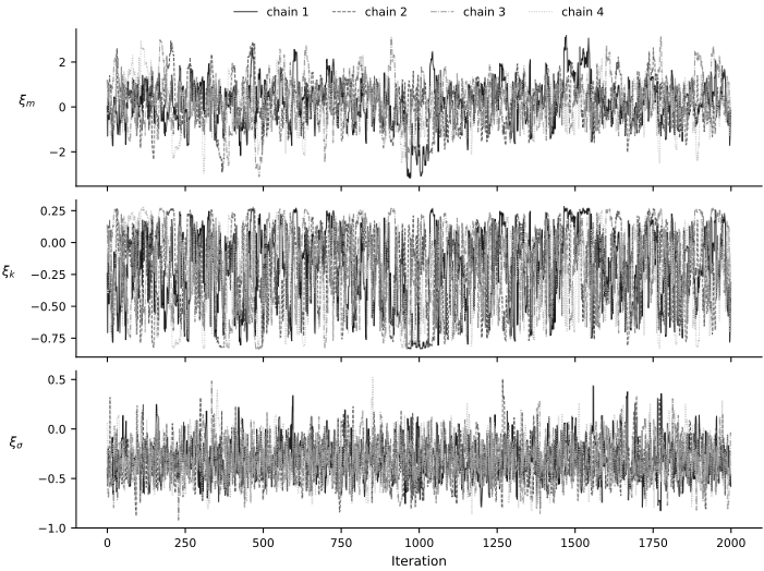
The unconstrained trace plots and diagnostics summarize how the four chains explore the posterior ridge.

Hide code cell source

fig, ax = plt.subplots(
    3, 1, sharex=True, figsize=FIGURE_SIZES["full_tall"], constrained_layout=True
)
for chain in range(posterior_samples_nuts_xi.shape[0]):
    color, linestyle = CHAIN_STYLES[chain]
    for coordinate in range(3):
        ax[coordinate].plot(
            posterior_samples_nuts_xi[chain, :, coordinate],
            color=color,
            linestyle=linestyle,
            linewidth=0.65,
            rasterized=True,
            label=f"chain {chain + 1}" if coordinate == 0 else None,
        )
for coordinate, label in enumerate([r"$\xi_m$", r"$\xi_k$", r"$\xi_\sigma$"]):
    ax[coordinate].set_ylabel(label, rotation=0, labelpad=15)
ax[0].legend(ncol=4, loc="lower center", bbox_to_anchor=(0.5, 1.0))
ax[-1].set_xlabel("Iteration")
finalize_axes(ax, keep_box=False);

display_diagnostics(
    ["xi-m", "xi-k", "xi-sigma"],
    posterior_samples_nuts_xi,
    original_divergences,
)
CoordinateR-hatBulk ESSDivergences
xi-m1.0084780
xi-k1.0084800
xi-sigma1.00221950
Four-chain trace plots for the three unconstrained parameters of the nonidentifiable oscillator model.

The \(m\) and \(k\) coordinates drift slowly and remain strongly coupled as the chains move along the posterior ridge. This produces high autocorrelation and can make marginal summaries sensitive to incomplete exploration. These are practical sampling symptoms of geometry already established analytically; they are not the proof of structural nonidentifiability.
Hide code cell source

posterior_samples_df = pd.DataFrame(
    np.asarray(flat_original_samples),
    columns=[r"$\xi_1$", r"$\xi_2$", r"$\xi_3$"]
)

pair_grid = sns.pairplot(
    posterior_samples_df, 
    diag_kind="hist", 
    height=2, aspect=1, markers=".",
    plot_kws={"alpha": 0.2, "color": "0.15", "s": 8, "rasterized": True},
    diag_kws={"color": "0.7", "edgecolor": "black"},
    corner=True,
)
pair_grid.fig.set_size_inches(*FIGURE_SIZES["full_tall"]);
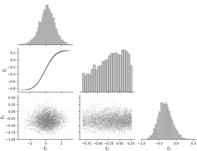
Pair plot of the unconstrained posterior showing the narrow dependence ridge.

The narrow band in the \((\xi_1,\xi_2)\) panel is the ridge expressed in unconstrained coordinates. Transforming the samples back to physical coordinates makes its meaning explicit.
Hide code cell source

posterior_samples_df = pd.DataFrame(
    np.column_stack(
        [
            posterior_samples_nuts.oscillator.m,
            posterior_samples_nuts.oscillator.k,
            posterior_samples_nuts.measurement.sigma,
        ]
    ),
    columns=[r"$m$", r"$k$", r"$\sigma$"]
)

pair_grid = sns.pairplot(
    posterior_samples_df, 
    diag_kind="hist", 
    height=2, aspect=1, markers=".",
    plot_kws={"alpha": 0.2, "color": "0.15", "s": 8, "rasterized": True},
    diag_kws={"color": "0.7", "edgecolor": "black"},
    corner=True,
)
pair_grid.fig.set_size_inches(*FIGURE_SIZES["full_tall"]);
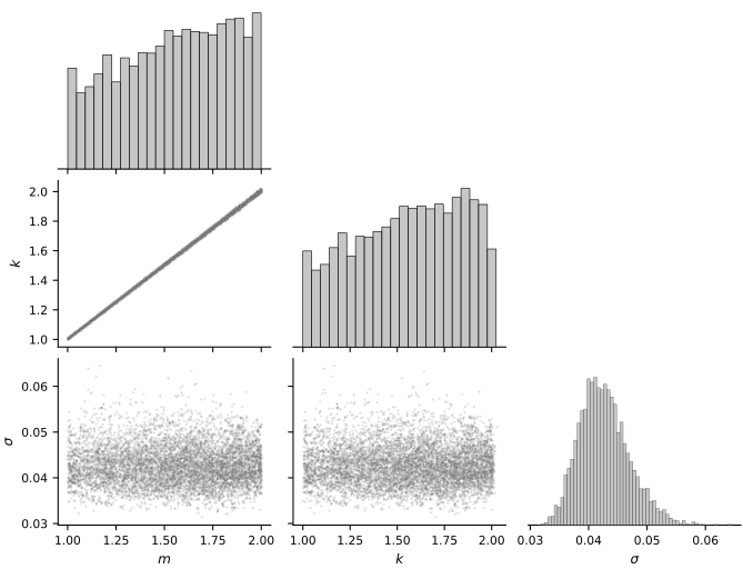
Pair plot in physical coordinates showing the posterior ridge between mass and stiffness.

For these data, the true ratio is \(k/m=1\), so the physical ridge lies near \(k=m\). More generally, it follows the line \(k=\omega^2m\). If the scientific objective requires \(m\) and \(k\) separately, the experiment needs independent information, such as a known mass or an additional force-response measurement.

Reduced model#

When only the oscillation frequency matters, we can replace \((m,k)\) by the identifiable combination \(\omega^2=k/m\). We assign the reduced model a new prior, \(\omega^2\sim\operatorname{Uniform}(0.25,3)\). This is a modeling choice, not the prior induced by the original independent uniform priors on \(m\) and \(k\).

Hide code cell source

# Containers for storing parameters
class ReparameterizedOscillatorParams(NamedTuple):
    omega2: float
    init_cond: OscillatorState

class ReparameterizedParams(NamedTuple):
    oscillator: ReparameterizedOscillatorParams
    measurement: MeasurementParams

class ReparameterizedParamsTransformation:
    def __init__(self, omega2_low, omega2_high, sigma_shift, sigma_scale, init_cond=None):
        self.omega2_low = omega2_low
        self.omega2_high = omega2_high
        self.sigma_shift = sigma_shift
        self.sigma_scale = sigma_scale
        self.init_cond = init_cond if init_cond is not None else OscillatorState(x=None, v=None)
        self.split_xi_fn = None
        params_tmp = ReparameterizedParams(
            oscillator=ReparameterizedOscillatorParams(
                omega2=0.5*(omega2_low + omega2_high), init_cond=self.init_cond
            ),
            measurement=MeasurementParams(sigma=jnp.exp(sigma_shift)),
        )
        xi_tmp = self.backward(params_tmp)  # This is just to set unflatten and split functions
        self._n_params = xi_tmp.shape[0]

    def forward(self, xi: ArrayLike) -> ReparameterizedParams:
        """Maps from unconstrained to constrained space."""
        osc_, meas_ = self.split_xi_fn(xi)

        # ODE model parameters
        omega2 = normal_to_uniform(osc_[0], self.omega2_low, self.omega2_high)
        osc = ReparameterizedOscillatorParams(omega2=omega2, init_cond=self.init_cond)

        # Measurement model parameters
        sigma = exp_transform(meas_[0], self.sigma_shift, self.sigma_scale)
        meas = MeasurementParams(sigma=sigma)

        return ReparameterizedParams(oscillator=osc, measurement=meas)
    
    def backward(self, p: ReparameterizedParams) -> Array:
        """Maps from constrained to unconstrained space."""
        # ODE model parameters
        xi_omega2 = uniform_to_normal(p.oscillator.omega2, self.omega2_low, self.omega2_high)
        xi_osc = jnp.hstack((xi_omega2,))
        
        # Measurement model parameters
        xi_sigma = log_transform(p.measurement.sigma, self.sigma_shift, self.sigma_scale)
        xi_meas = jnp.hstack((xi_sigma,))
        
        # Combine
        xi, f = ravel_pytree((xi_osc, xi_meas))
        if self.split_xi_fn is None:
            self.split_xi_fn = f
        
        return xi
    
    @property
    def n_params(self):
        return self._n_params

def reparameterized_harmonic_oscillator(
    t: ArrayLike, 
    params: ReparameterizedOscillatorParams
) -> OscillatorState:
    """Analytic solution to the harmonic oscillator ODE system."""
    init = params.init_cond
    omega = params.omega2**0.5
    position = init.x*jnp.cos(omega*t) + init.v/omega*jnp.sin(omega*t)
    velocity = -init.x*omega*jnp.sin(omega*t) + init.v*jnp.cos(omega*t)
    return OscillatorState(x=position, v=velocity)
T_re = ReparameterizedParamsTransformation(
    omega2_low=0.25,
    omega2_high=3.0,
    sigma_shift=-3,
    sigma_scale=0.5,
    init_cond=OscillatorState(x=1.0, v=0.0)
)

reparameterized_prob_model = ProbabilisticDynamicalSystem(
    T_re, reparameterized_harmonic_oscillator
)
reparameterized_log_posterior_wrapped = partial(
    reparameterized_prob_model.log_posterior,
    obs_times=obs_times,
    obs_positions=obs_positions,
)
initial_positions_re = jnp.array(
    [
        [-0.85, -0.4],
        [-0.70, 0.0],
        [-0.55, 0.4],
        [-0.40, 0.2],
    ]
)
posterior_samples_nuts_xi_re, reduced_divergences = run_nuts_chains(
    reparameterized_log_posterior_wrapped,
    initial_positions_re,
    key=jrandom.PRNGKey(20260920),
)
flat_reduced_samples = posterior_samples_nuts_xi_re.reshape((-1, T_re.n_params))
posterior_samples_nuts_re = vmap(T_re.forward)(flat_reduced_samples)

Hide code cell source

fig, ax = plt.subplots(
    2, 1, sharex=True, figsize=FIGURE_SIZES["full_standard"], constrained_layout=True
)
for chain in range(posterior_samples_nuts_xi_re.shape[0]):
    color, linestyle = CHAIN_STYLES[chain]
    for coordinate in range(2):
        ax[coordinate].plot(
            posterior_samples_nuts_xi_re[chain, :, coordinate],
            color=color,
            linestyle=linestyle,
            linewidth=0.65,
            rasterized=True,
            label=f"chain {chain + 1}" if coordinate == 0 else None,
        )
ax[0].set_ylabel(r"$\xi_{\omega^2}$", rotation=0, labelpad=20)
ax[1].set_ylabel(r"$\xi_\sigma$", rotation=0, labelpad=15)
ax[0].legend(ncol=4, loc="lower center", bbox_to_anchor=(0.5, 1.0))
ax[-1].set_xlabel("Iteration")
finalize_axes(ax, keep_box=False);

display_diagnostics(
    ["xi-omega2", "xi-sigma"],
    posterior_samples_nuts_xi_re,
    reduced_divergences,
)
CoordinateR-hatBulk ESSDivergences
xi-omega21.00242040
xi-sigma1.00329900
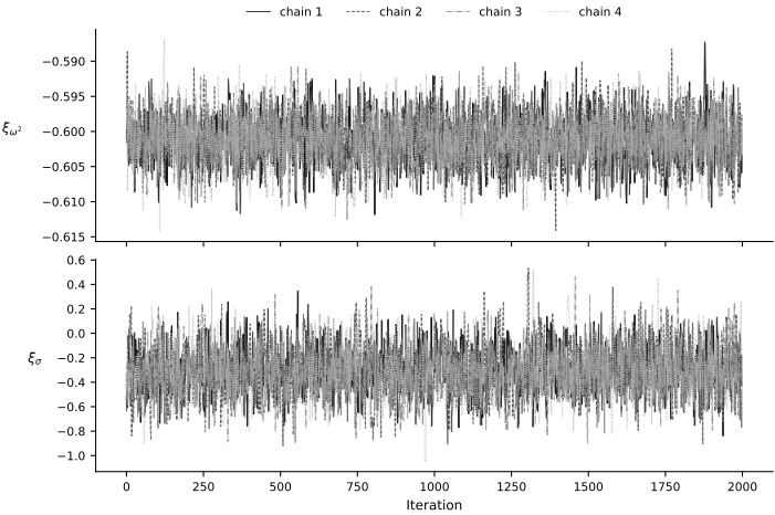
Four-chain trace plots for frequency squared and noise scale in the reduced model.

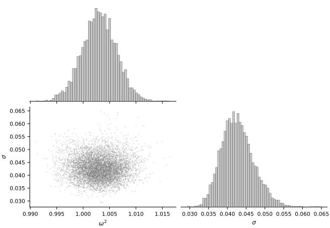
The reduced posterior has no \(m\)–\(k\) ridge. The trace plots and diagnostics now assess the numerical exploration of this two-parameter posterior; the structural conclusion still comes from the analytic dependence of the trajectory on \(\omega^2\).
Hide code cell source

posterior_samples_df_re = pd.DataFrame(
    np.column_stack(
        [
            posterior_samples_nuts_re.oscillator.omega2,
            posterior_samples_nuts_re.measurement.sigma,
        ]
    ),
    columns=[r"$\omega^2$", r"$\sigma$"]
)

pair_grid = sns.pairplot(
    posterior_samples_df_re, 
    diag_kind="hist", 
    height=2.5, aspect=1, markers=".",
    plot_kws={"alpha": 0.2, "color": "0.15", "s": 8, "rasterized": True},
    diag_kws={"color": "0.7", "edgecolor": "black"},
    corner=True,
)
pair_grid.fig.set_size_inches(*FIGURE_SIZES["full_standard"]);
Pair plot of the reduced posterior for frequency squared and noise scale.

With the known nonzero initial displacement used here, an ideal continuous noise-free position trajectory determines \(\omega^2\) on the stated positive parameter range. Finite noisy observations can still make \(\omega^2\) practically difficult to estimate, and sparse sampling can alias different frequencies. The distinction between structural and practical identifiability therefore remains essential.