Symbolic Differentiation

Symbolic differentiation mimics programmatically what you do by hand when calculating derivatives. It works by building up a representation of the mathematical expression that you want to differentiate. This is called an expression tree. Expression trees are made out of nodes that can be either operators or operands. Operators are things like +, -, *, /, or functions like sin, cos, exp, log, etc. Operands are things like numbers, variables, or other expressions.

For example, the expression:

\[ f(x) = 1 + x^2 \]

would be represented by the following expression tree. The diagrams use shaded rounded rectangles for operators and unfilled ellipses for operands. The label sqr denotes squaring, and pow denotes exponentiation.

Show code cell source

Hide code cell source

import base64

import graphviz
from IPython.display import display

g = graphviz.Digraph(
    graph_attr={"bgcolor": "transparent", "margin": "0.02", "ordering": "out"},
    node_attr={
        "fontname": "DejaVu Sans", "fontsize": "9",
        "color": "black", "penwidth": "1.0",
    },
    edge_attr={"arrowhead": "none", "color": "black", "penwidth": "0.8"},
)

operator_node = {
    "shape": "box", "style": "rounded,filled",
    "fillcolor": "gray85", "color": "black",
}
operand_node = {
    "shape": "ellipse", "style": "filled",
    "fillcolor": "white", "color": "black",
}

def display_graph(graph):
    """Display vector web output and print-compatible PDF/PNG fallbacks."""
    svg = graph.pipe(format="svg").decode("utf-8")
    pdf = graph.pipe(format="pdf")
    graph.graph_attr["dpi"] = "300"
    try:
        png = graph.pipe(format="png")
    finally:
        graph.graph_attr.pop("dpi", None)
    display(
        {
            "image/svg+xml": svg,
            "application/pdf": base64.b64encode(pdf).decode("ascii"),
            "image/png": base64.b64encode(png).decode("ascii"),
        },
        raw=True,
    )

g.node('+', **operator_node)
g.node('sqr', **operator_node)
g.node('1', **operand_node)
g.node('x', **operand_node)
g.edge('+', '1')
g.edge('+', 'sqr')
g.edge('sqr', 'x')
display_graph(g)

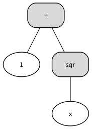
Here is an expression tree for:

\[ f(x,y) = \left(\frac{\sin x}{x}\right)^2 + y^3. \]

Show code cell source

Hide code cell source

g = graphviz.Digraph(
    graph_attr={"bgcolor": "transparent", "margin": "0.02", "ordering": "out"},
    node_attr={
        "fontname": "DejaVu Sans", "fontsize": "9",
        "color": "black", "penwidth": "1.0",
    },
    edge_attr={"arrowhead": "none", "color": "black", "penwidth": "0.8"},
)

g.node('+', **operator_node)
g.node('sqr', **operator_node)
g.node('sin', **operator_node)
g.node('pow', **operator_node)
g.node('/', **operator_node)
g.node('3', **operand_node)
# make two different nodes for x
g.node('x1', label='x', **operand_node)
g.node('x2', label='x', **operand_node)
g.node('y', **operand_node)

g.edge('sin', 'x1')
g.edge('/', 'sin')
g.edge('/', 'x2')
g.edge('sqr', '/')
g.edge('+', 'sqr')
g.edge('+', 'pow')
g.edge('pow', 'y')
g.edge('pow', '3')

display_graph(g)

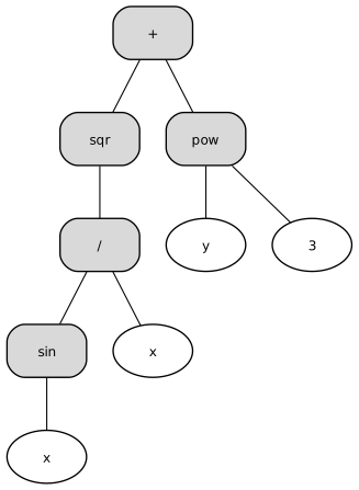
You get the idea.

One of the first things that we would like to do is evaluate the expression. Here is pseudocode for how to evaluate an expression tree:

    def evaluate(node):
        if node is an operator:
            evaluate the operands
            apply the operator to the operands
            return the result
        else:
            return the value of the operand

Similarly, we can write generic code to differentiate an expression tree with respect to a variable. To write such code, we need to know the derivative of each operator and the chain rule. For example, the derivative of the addition operator is:

\[ \partial_x (f + g) = \partial_x f + \partial_x g. \]

Here we are using the notation \(\partial_x f\) to mean the partial derivative of \(f\) with respect to the variable \(x\), i.e., \(\partial_x f = \frac{\partial f}{\partial x}\).

Similarly, for the multiplication operator:

\[ \partial_x (f g) = f \partial_x g + g \partial_x f. \]

And so on for all operators.

Equipped with these basic operations, we can write a generic function to differentiate an expression tree with respect to a variable:

    def differentiate(node, variable):
        if node is an operator:
            differentiate the operands
            apply the derivative rule for the operator to the operands
            return the result
        else:
            if node is the variable:
                return 1
            else:
                return 0

For a deeper treatment, see Structure and Interpretation of Computer Programs (Abelson et al., 1996).

The Python package sympy is a library for symbolic mathematics. Let’s use it to build these trees.

import sympy
from sympy.abc import x, y

f = (sympy.sin(x) / x) ** 2 + y ** 3

f

\[\displaystyle y^{3} + \frac{\sin^{2}{\left(x \right)}}{x^{2}}\]

Here is the expression tree as it is internally represented by sympy.

sympy.srepr(f)

"Add(Pow(Symbol('y'), Integer(3)), Mul(Pow(Symbol('x'), Integer(-2)), Pow(sin(Symbol('x')), Integer(2))))"

You can evaluate the expression tree:

f.evalf(subs={x: 1, y: 2})

\[\displaystyle 8.70807341827357\]

Or you can make a python function that evaluates the expression tree at any point:

f_func = sympy.lambdify([x, y], f)

f_func(1, 2)

np.float64(8.708073418273571)

And of course, you can differentiate the expression tree:

# Differentiate with respect to x
pxf = f.diff(x)
pxf

\[\displaystyle \frac{2 \sin{\left(x \right)} \cos{\left(x \right)}}{x^{2}} - \frac{2 \sin^{2}{\left(x \right)}}{x^{3}}\]

And you can evaluate that anywhere you want:

pxf_func = sympy.lambdify([x, y], pxf)

pxf_func(1, 2)

np.float64(-0.5068494097214605)

There are two main problems with symbolic differentiation. Loops and conditionals are difficult to handle symbolically, which restricts the class of functions we can differentiate. In addition, expression trees can grow very large very quickly, a phenomenon called expression swell. We begin with the softplus function, a smooth approximation to \(\max(0,z)\):

w, b = sympy.symbols('w b')
# Softplus
f = sympy.log(1 + sympy.exp(w * x + b))
f

\[\displaystyle \log{\left(e^{b + w x} + 1 \right)}\]

Here is the gradient of this function with respect to \(w\):

f.diff(w)

\[\displaystyle \frac{x e^{b + w x}}{e^{b + w x} + 1}\]

Now let’s nest the softplus function a few more times:

f2 = sympy.log(1 + sympy.exp(w * f + b))
f2

\[\displaystyle \log{\left(e^{b + w \log{\left(e^{b + w x} + 1 \right)}} + 1 \right)}\]

Here is the derivative now:

f2.diff(w)

\[\displaystyle \frac{\left(\frac{w x e^{b + w x}}{e^{b + w x} + 1} + \log{\left(e^{b + w x} + 1 \right)}\right) e^{b + w \log{\left(e^{b + w x} + 1 \right)}}}{e^{b + w \log{\left(e^{b + w x} + 1 \right)}} + 1}\]

Okay, one more time to make the point:

f3 = sympy.log(1 + sympy.exp(w * f2 + b))
f3

\[\displaystyle \log{\left(e^{b + w \log{\left(e^{b + w \log{\left(e^{b + w x} + 1 \right)}} + 1 \right)}} + 1 \right)}\]

Expanding \(\partial_w f_3\) into one line repeats every inner function and derivative. Define \(\sigma(z)=e^z/(1+e^z)\), the derivative of the softplus. Keeping the intermediate names \(f\) and \(f_2\) exposes the same calculation without printing the unwieldy expansion:

\[\begin{split} \begin{aligned} \partial_w f &= \sigma(b+wx)x,\\ \partial_w f_2 &= \sigma(b+wf)\left(f+w\partial_w f\right),\\ \partial_w f_3 &= \sigma(b+wf_2)\left(f_2+w\partial_w f_2\right). \end{aligned} \end{split}\]

After substituting the intermediate definitions, the SymPy strings for \(\partial_w f\), \(\partial_w f_2\), and \(\partial_w f_3\) grow from 33 to 133 to 293 characters, while their operation counts grow from 9 to 35 to 76. A fourth layer would copy the same nested structure again.

derivatives = (f.diff(w), f2.diff(w), f3.diff(w))
for name, derivative in zip(("f", "f2", "f3"), derivatives):
    print(
        f"d{name}/dw: {len(str(derivative))} characters, "
        f"{sympy.count_ops(derivative)} operations"
    )

df/dw: 33 characters, 9 operations
df2/dw: 133 characters, 35 operations
df3/dw: 293 characters, 76 operations

This growth of the fully substituted derivative is the expression swell problem. Automatic differentiation avoids materializing one global symbolic formula; it propagates local derivative rules through a computational graph.