Spectral Bias of Neural Networks#
Rahaman et al. (2019) showed that neural networks are biased toward low-frequency components of the input signal. This behavior is known as spectral bias. This problem inhibits the ability to train PINNs for high frequency problems, e.g., problems exhibiting localized features like shocks, boundary layers, etc. The problem of spectral bias can be understood theoretically using the neural tangent kernel (NTK), which describes how small parameter updates near initialization change the network’s predictions. We will demonstrate this bias using a simple example. We will train a simple MLP to approximate a function with a low frequency and a high frequency component. We will check how the MLP does after each epoch. You should notice that the MLP is biased towards the low frequency component of the function. Only after a large number of epochs, the MLP starts to capture the high frequency component of the function.
Numerical Example#
The function we will use is given by
for \(x \in [0, 1]\).
Let’s visualize it and the data we will use for training the neural network.
import numpy as np
import jax.numpy as jnp

f = lambda x: jnp.sin(2.0 * jnp.pi * x) + 0.5 * jnp.sin(16.0 * jnp.pi * x)

num_train = 1_000
x_train = np.random.rand(num_train)
y_train = f(x_train) + np.random.randn(num_train) * 0.1

fig, ax = plt.subplots(figsize=FIGURE_SIZES["half_standard"])
x = jnp.linspace(0, 1, 100)
ax.plot(x, f(x), 'r-', label='True function')
ax.scatter(x_train, y_train, s=4, c='black', alpha=0.5, label='Training data')
ax.set_xlabel(r"$x$")
ax.set_ylabel(r"$f(x)$")
ax.legend(loc='best', frameon=True)
finalize_axes(keep_box=False)
array([<Axes: xlabel='$x$', ylabel='$f(x)$'>], dtype=object)
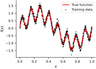
The following code trains a generic neural network on the data. It returns the trained model after each epoch.
Let’s also write some code to visualize the predictions of the model after each epoch.
We will try this on a simple MLP:
import jax.random as jrandom

key = jrandom.PRNGKey(0)
subkey, key = jrandom.split(key)

width_size = 128
depth = 4
mlp = eqx.filter_vmap(
    eqx.nn.MLP(1, 1, width_size, depth, jnp.tanh, key=subkey))

optimizer = optax.adam(1e-3)
model, path, losses = train_batch(
    mlp, x_train, y_train, optimizer,
    n_batch=32,
    n_epochs=300,
    freq=1_000
)
Now, let’s plot the result after some of the epochs:
for e, model in enumerate(path[::50]):
    fig, ax = plot(model, x_train, y_train, f)
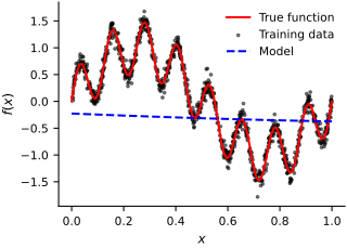
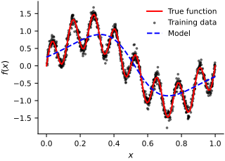
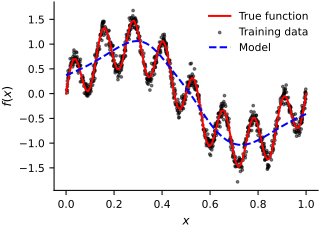
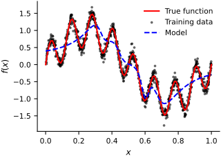
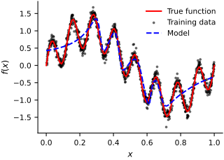
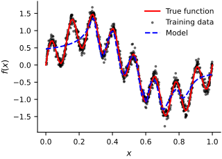
And you clearly observe the spectral bias problem.
Random Fourier Features#
One way to mitigate spectral bias is to use random Fourier features (Tancik et al., 2020). The idea is to map the input data to a higher dimensional space using random Fourier features. The random Fourier features are designed to capture the high frequency components of the input signal. These features go right before the input layer of the neural network. Say our input data is \(\mathbf{x} \in \mathbb{R}^d\) and that we want to map to a network with \(2m\)-dimensional inputs. Then, the random Fourier features are given by
where \(\mathbf{B}\) is an \(m \times d\) matrix. This matrix is constant throughout the training process. But we typically pick it randomly from a Gaussian distribution. Specifically, we pick each entry of \(\mathbf{B}\) from a Gaussian distribution with mean 0 and variance \(\sigma^2\). Wang et al. (2023) recommend moderately large values of \(\sigma\) between \(1\) and \(10\) for PINNs. This range is a problem-dependent starting point rather than a universal rule. The cosine and sine functions are applied element-wise.
Applying Random Fourier Features to the Example#
Let’s implement random Fourier features and apply it to the previous example.
import jax
from functools import partial
import jax.tree_util as jtu


class FourierEncoding(eqx.Module):
    B: jax.Array

    @property
    def num_fourier_features(self) -> int:
        return self.B.shape[0]

    @property
    def in_size(self) -> int:
        return self.B.shape[1]

    @property
    def out_size(self) -> int:
        return self.B.shape[0] * 2

    def __init__(self,
                 in_size: int,
                 num_fourier_features: int,
                 key: jax.random.PRNGKey,
                 sigma: float = 1.0):
        self.B = jax.random.normal(
            key, shape=(num_fourier_features, in_size),
            dtype=jax.numpy.float32) * sigma

    def __call__(self, x: jax.Array) -> jax.Array:
        return jax.numpy.concatenate(
            [jax.numpy.cos(jax.numpy.dot(self.B, x)),
             jax.numpy.sin(jax.numpy.dot(self.B, x))],
            axis=0)
And here is how we can make the network.
num_fourier_features = 100
width_size = 128
depth = 4
sigma = 5.0

key1, key2, key = jax.random.split(key, 3)
fourier = FourierEncoding(1, num_fourier_features, key1, sigma)
mlp = eqx.nn.MLP(fourier.out_size, 1, width_size, depth, jax.numpy.tanh, key=key2)
fourier_mlp = eqx.filter_vmap(eqx.nn.Sequential([eqx.nn.Lambda(fourier), eqx.nn.Lambda(mlp)]))
Recall that we want to keep \(\mathbf{B}\) constant throughout the training process.
We will have to modify our training algorithm to achieve this.
We will use equinox.partition capabilities to achieve this.
filter_spec = jtu.tree_map(lambda _: True, fourier_mlp)
filter_spec = eqx.tree_at(
    lambda tree: (tree._fun[0].fn.B,),
    filter_spec,
    replace=(False,),
)
def train_fourier(
        model,
        x, y,
        optimizer,
        filter_spec,
        n_batch=10,
        n_epochs=10,
        freq=1_000,
    ):

    # A new loss is also needed
    # It needs to combine the part of the model over
    # which we optimize with the part where we don't
    def new_loss(diff_model, static_model, x, y):
            comb_model = eqx.combine(diff_model, static_model)
            return loss(comb_model, x, y)

    # This is the step of the optimizer. We **always** jit:
    @eqx.filter_jit
    def step(opt_state, model, xi, yi):
        # The next two lines are also different
        # First we split the model into two parts
        diff_model, static_model = eqx.partition(model, filter_spec)
        # Then, we call the new loss
        value, grads = eqx.filter_value_and_grad(new_loss)(diff_model, static_model, xi, yi)
        updates, opt_state = optimizer.update(grads, opt_state)
        model = eqx.apply_updates(model, updates)
        return model, opt_state, value

    # The state of the optimizer
    opt_state = optimizer.init(eqx.filter(model, eqx.is_inexact_array))
    # The path of the model
    path = []
    # The path of the test loss
    losses = []
    for e in range(n_epochs):
        for i, (xb, yb) in enumerate(data_generator(x, y, n_batch)):
            model, opt_state, value = step(opt_state, model, xb[:, None], yb)
            if i % freq == 0:
                path.append(model)
                losses.append(value)
                print(f"Epoch {e}, step {i}, loss {value:.3f}, test {losses[-1]:.3f}")
    return model, path, losses
Let’s train it just for 100 epochs.
optimizer = optax.adam(1e-3)
trained_v_fourier_model, fourier_path, losses = train_fourier(
    fourier_mlp, x_train, y_train, optimizer,
    filter_spec,
    n_batch=32,
    n_epochs=100,
    freq=1_000
)
Here are the results:
for e, model in enumerate(fourier_path[::10]):
    fig, ax = plot(model, x_train, y_train, f, style='g-.')
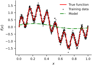
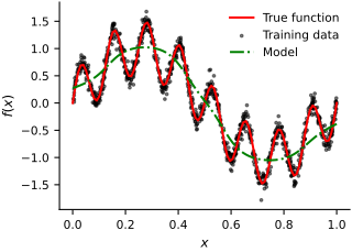
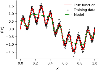
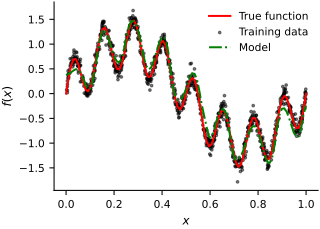
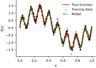
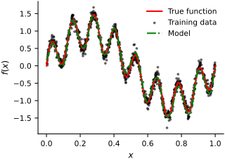
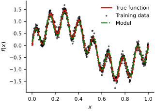
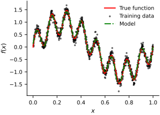
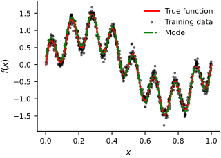
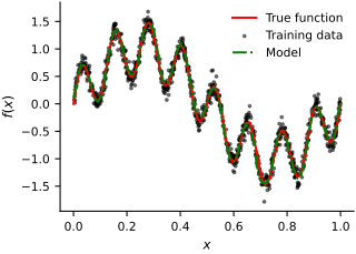
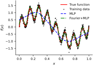
Notice that we learn the high-frequency component much faster than before. Let’s compare the two models side by side.
fig, ax = plt.subplots(figsize=FIGURE_SIZES["half_standard"])
x = jnp.linspace(0, 1, 100)[:, None]
ax.plot(x, f(x), 'r-', label='True function')
ax.scatter(x_train, y_train, s=4, c='black', alpha=0.5, label='Training data')
ax.plot(x, path[99](x), 'b--', label='MLP')
ax.plot(x, fourier_path[99](x), 'g-.', label='Fourier+MLP')
ax.set_xlabel(r"$x$")
ax.set_ylabel(r"$f(x)$")
plt.legend(loc='best', frameon=False);
finalize_axes(keep_box=False)
array([<Axes: xlabel='$x$', ylabel='$f(x)$'>], dtype=object)
PINNs with Random Fourier Features#
Let’s now see if we can do any better with PINNs on our steady-state heat equation example.
Let’s build everything to train the model. Notice that we need to rescale.
from jax import grad, vmap

u0 = 500 # degrees Kelvin
k = 10.0 # thermal conductivity in W/mK
Lx = 0.1 # meters
Ly = 1.0 # meters

to_x = lambda xt: xt * Lx
to_y = lambda yt: yt * Ly
to_xt = lambda x: x / Lx
to_yt = lambda y: y / Ly

source_term = lambda x, y: 2.0 * jnp.pi ** 2 * k * u0 * (
    -Lx ** 2 * jnp.sin(jnp.pi * x / Lx) ** 2 * jnp.cos(2.0 * jnp.pi * y / Ly)
    -Ly ** 2 * jnp.sin(jnp.pi * y / Ly) ** 2 * jnp.cos(2.0 * jnp.pi * x / Lx)
) / (Lx ** 2 * Ly ** 2)

key1, key2, key = jax.random.split(key, 3)
num_fourier_features = 100
width_size = 128
depth = 4

model = eqx.nn.Sequential([
    eqx.nn.Lambda(
        FourierEncoding(2, num_fourier_features, key1, sigma=6.0)),
    eqx.nn.Lambda(
        eqx.nn.MLP(num_fourier_features * 2, 1, width_size, depth, jnp.tanh, key=key2)),
    eqx.nn.Lambda(
        lambda y: y[0])])
# remember that we need a way to filter out the parameters of the Fourier encoding
filter_spec = jtu.tree_map(lambda _: True, model)
filter_spec = eqx.tree_at(
    lambda tree: (tree[0].fn.B,),
    filter_spec,
    replace=(False,))

# The model that satisfies the boundary conditions
u_hat = lambda x, y, model: x * (1.0 - x) * y * (1.0 - y) * model(jnp.array([x, y]))
u_x = grad(u_hat, 0)
u_y = grad(u_hat, 1)
u_xx = grad(u_x, 0)
u_yy = grad(u_y, 1)

# We need to find new scaling factors because the network structure has changed
v_u_xx = eqx.filter_jit(eqx.filter_vmap(u_xx, in_axes=(0, 0, None)))
v_u_yy = eqx.filter_jit(eqx.filter_vmap(u_yy, in_axes=(0, 0, None)))
x = jnp.linspace(0, Lx, 100)
y = jnp.linspace(0, Ly, 100)
X, Y = jnp.meshgrid(x, y)
Xt = to_xt(X)
Yt = to_yt(Y)
max_u_xx = jnp.abs(v_u_xx(Xt.flatten(), Yt.flatten(), model)).max()
max_u_yy = jnp.abs(v_u_yy(Xt.flatten(), Yt.flatten(), model)).max()

# Calculate the scale:
fs = 9.96e+06
us = fs / k / max(max_u_xx, max_u_yy) / max(1/Lx**2, 1/Ly**2)
tkx = (k * us) / (Lx ** 2 * fs)
tky = (k * us) / (Ly ** 2 * fs)

print(f"Scale factor fs: {fs:.2e}")
print(f"Scale factor us: {us:.2e}")
print(f"tkx = {tkx:.3e}, tky = {tky:.3e}")

tilde_source_term = lambda tx, ty: source_term(to_x(tx), to_y(ty)) / fs

pde_residual = vmap(
    lambda x, y, model: tkx * u_xx(x, y, model) + tky * u_yy(x, y, model) + tilde_source_term(x, y),
    in_axes=(0, 0, None))
pinn_loss = lambda model, x, y: jnp.mean(jnp.square(pde_residual(x, y, model)))
Scale factor fs: 9.96e+06
Scale factor us: 2.69e+04
tkx = 2.704e+00, tky = 2.704e-02
This is how we train:
key, subkey = jax.random.split(key)
optimizer = optax.adam(1e-3)
trained_model, losses = train_pinn(
    pinn_loss, model, key, optimizer, filter_spec,
    num_collocation_residual=256, num_iter=2_000, freq=100, Lx=1.0, Ly=1.0)
Step 0, residual loss 2.737e-01
Step 100, residual loss 1.276e-04
Step 200, residual loss 5.678e-05
Step 300, residual loss 2.237e-05
Step 400, residual loss 2.082e-05
Step 500, residual loss 1.701e-05
Step 600, residual loss 1.265e-05
Step 700, residual loss 1.450e-05
Step 800, residual loss 1.697e-05
Step 900, residual loss 3.733e-05
Step 1000, residual loss 3.822e-05
Step 1100, residual loss 5.602e-05
Step 1200, residual loss 1.472e-04
Step 1300, residual loss 2.336e-05
Step 1400, residual loss 1.895e-05
Step 1500, residual loss 5.885e-06
Step 1600, residual loss 1.271e-05
Step 1700, residual loss 8.260e-06
Step 1800, residual loss 1.379e-04
Step 1900, residual loss 1.152e-05
Save the loss for later use:
import numpy as np
np.savez("fourier_mlp_losses.npz", losses=losses)
Note
Training time depends on the available hardware and includes the initial JAX compilation.
We now compare with the plain MLP.
import numpy as np
mlp_losses = np.load("mlp_losses.npz")["losses"]
fig, ax = plt.subplots(figsize=FIGURE_SIZES["half_standard"])
ax.plot(mlp_losses, label="MLP")
ax.plot(losses, '--', label="MLP+Fourier")
# set log scale for y axis
ax.set_yscale('log')
ax.set_xlabel("Iterations x 100")
ax.set_ylabel("Loss")
plt.legend(loc="best", frameon=False)
finalize_axes(keep_box=False)
array([<Axes: xlabel='Iterations x 100', ylabel='Loss'>], dtype=object)
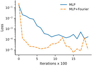
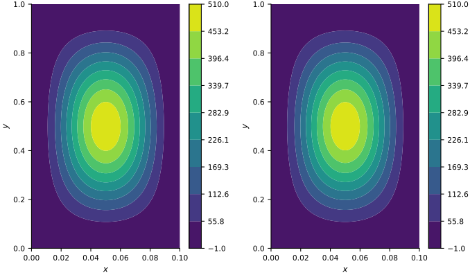
Here is the solution we found compared to the exact solution:
And here is the error:
array([<Axes: xlabel='x', ylabel='y'>, <Axes: label='<colorbar>'>],
      dtype=object)