Example: 3D Particle Position Reconstruction from Images

This example implements a small synthetic version of the stochastic volumetric reconstruction method of Hans et al. (2023).

The paper proposes a Bayesian reconstruction method for 3D particle locations from synchronized multi-camera images. Its predicted intensity on camera \(m\) is

\[ f_m(z) = I_0 \sum_{n=1}^N \exp\left(-\frac{\|z - h_m(x_n)\|^2}{2\sigma_{\mathrm{img}}^2}\right), \]

where:

• \(x_n \in \mathbb{R}^3\) are candidate particle positions,

• \(h_m\) is the calibration map for camera \(m\),

• \(z \in \mathbb{R}^2\) is a location on the image plane of camera \(m\), \(I_0\) is the peak particle intensity, and \(\sigma_{\mathrm{img}}\) is the image-plane blob width.

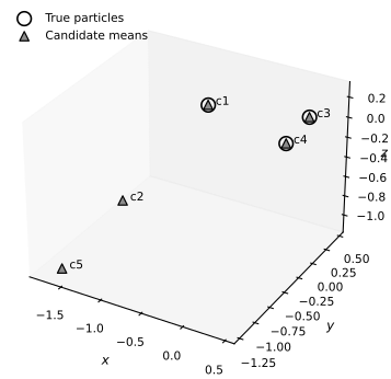
As in the paper, we deliberately use more candidate particles than the true number of particles. Variational inference then tries to explain the images while an additional quadratic term encourages unnecessary particles to drift away from the imaging region.

Simplifications in this teaching example

We keep the main structure of the method, but simplify several parts:

• We use three synthetic cameras with linear projection maps instead of a full laboratory calibration model.

• We use a diagonal Gaussian guide for the candidate particle locations.

• We optimize a Monte Carlo estimate of the ELBO with Adam.

• After optimization, we cluster nearby candidates to remove duplicates and identify the reconstructed particles.

These simplifications retain the variational reconstruction of a sparse 3D particle field directly from image data.

Synthetic multi-camera dataset

We place three particles in a cubic domain and render them onto three cameras. Each particle contributes a Gaussian blob on every image plane. We then add independent, zero-mean Gaussian pixel noise and treat the resulting images as observations. We retain negative noisy intensities in the likelihood and use a zero lower intensity limit only for display. The resulting observations are shown in Fig. 23.

height = 20
width = 20
num_true_particles = 3
num_candidate_particles = 5

peak_intensity = 0.8
particle_spread = 0.9
noise_std = 0.01

prior_scale = 2.0
penalty_strength = 0.5
repulsion_strength = 0.05
repulsion_length = 0.06

learning_rate = 3e-3
num_steps = 2500
num_mc_samples = 32

camera_matrices = jnp.array(
    [
        [[1.00, 0.00, 0.00], [0.00, 1.00, 0.00]],
        [[0.85, 0.10, 0.55], [0.02, 0.95, 0.22]],
        [[0.93, -0.18, 0.34], [0.06, 0.90, 0.48]],
    ],
    dtype=jnp.float64,
)

true_positions = jnp.array(
    [
        [-0.55, -0.20, 0.25],
        [-0.05, 0.45, -0.35],
        [0.45, 0.10, 0.20],
    ],
    dtype=jnp.float64,
)

row_coords, col_coords = jnp.meshgrid(
    jnp.arange(height), jnp.arange(width), indexing="ij"
)
pixel_grid = jnp.stack([col_coords, row_coords], axis=-1)


def project_points(points, camera_matrix):
    projected = points @ camera_matrix.T
    scale = jnp.array([width - 1, height - 1], dtype=jnp.float64)
    return 0.5 * (projected + 1.0) * scale


def render_camera(points, camera_matrix):
    uv = project_points(points, camera_matrix)
    displacement = pixel_grid[None, :, :, :] - uv[:, None, None, :]
    sqdist = jnp.sum(displacement**2, axis=-1)
    blobs = jnp.exp(-0.5 * sqdist / particle_spread**2)
    return peak_intensity * jnp.sum(blobs, axis=0)


def render_all_cameras(points):
    return jax.vmap(lambda camera_matrix: render_camera(points, camera_matrix))(
        camera_matrices
    )


clean_images = render_all_cameras(true_positions)
observed_images = clean_images + noise_std * jr.normal(jr.PRNGKey(1), clean_images.shape)
# Keep Gaussian observations unbounded for inference.
# The imshow limits below affect the display only.


fig, axes = plt.subplots(
    1,
    3,
    figsize=FIGURE_SIZES["full_landscape"],
    sharex=True,
    sharey=True,
    constrained_layout=True,
)
intensity_limit = float(jnp.max(observed_images))
for idx, ax in enumerate(axes):
    image = ax.imshow(
        observed_images[idx],
        origin="lower",
        cmap="Greys",
        vmin=0.0,
        vmax=intensity_limit,
        interpolation="nearest",
    )
    ax.set_title(f"Camera {idx + 1}")
    ax.set_xlabel("pixel $x$")
axes[0].set_ylabel("pixel $y$")
colorbar = fig.colorbar(image, ax=axes, fraction=0.035, pad=0.02)
colorbar.set_label("Observed intensity")
finalize_axes(axes, keep_box=True)
plt.show()

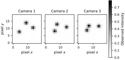
Fig. 23 Synthetic observations of the same three particles from three camera directions. A common grayscale maps pixel intensity across the images.

During inference we treat the particle coordinates used to generate the synthetic data as unknown and instead optimize an approximate posterior over an overcomplete set of five candidate particles.

Variational formulation

Let \(X = (x_1, \dots, x_N)\) denote the candidate particle locations and let \(M\) be the number of cameras. We use the generative model

\[ p(Y \mid X) = \prod_{m=1}^M \prod_{r,c} \mathcal{N}\left( Y_{mrc} \mid f_m(X)_{rc}, \sigma_\text{noise}^2 \right), \]

together with a weak Gaussian prior on each coordinate. The guide is a diagonal Gaussian

\[ q_\phi(X) = \prod_{n=1}^N \prod_{\ell=1}^3 \mathcal{N}(x_{n\ell} \mid \mu_{n\ell}, s_{n\ell}^2). \]

Following the spirit of the paper, we add a positive quadratic term to the ELBO so that candidate particles that are not needed are encouraged to move away from the domain:

\[ \mathcal{L}_{\text{aug}}(\phi) = \mathbb{E}_{q_\phi}[\log p(Y, X) - \log q_\phi(X)] + \varepsilon \mathbb{E}_{q_\phi}\left[ \frac{1}{3N} \sum_{n=1}^N \|x_n\|_2^2 \right]. \]

In this synthetic example we also include a very small repulsion term between candidates so that duplicate particles are less attractive numerically.

def unpack_variational_params(phi):
    num_coordinates = num_candidate_particles * 3
    mu = phi[:num_coordinates].reshape(num_candidate_particles, 3)
    log_std = phi[num_coordinates:].reshape(num_candidate_particles, 3)
    return mu, log_std


def pairwise_repulsion(points):
    differences = points[:, None, :] - points[None, :, :]
    sqdist = jnp.sum(differences**2, axis=-1)
    mask = 1.0 - jnp.eye(points.shape[0])
    return jnp.sum(jnp.exp(-sqdist / repulsion_length) * mask) / (
        points.shape[0] * (points.shape[0] - 1)
    )


def augmented_elbo(phi, key):
    mu, log_std = unpack_variational_params(phi)
    std = jnp.exp(log_std)

    epsilon = jr.normal(
        key, (num_mc_samples, num_candidate_particles, 3), dtype=jnp.float64
    )
    samples = mu[None, :, :] + std[None, :, :] * epsilon

    rendered_images = jax.vmap(render_all_cameras)(samples)
    residual = observed_images - rendered_images
    log_likelihood = -0.5 * jnp.sum(
        (residual / noise_std) ** 2, axis=(1, 2, 3)
    )
    log_likelihood -= observed_images.size * jnp.log(
        jnp.sqrt(2.0 * jnp.pi) * noise_std
    )

    log_prior = -0.5 * jnp.sum((samples / prior_scale) ** 2, axis=(1, 2))
    log_prior -= samples.shape[1] * samples.shape[2] * jnp.log(
        jnp.sqrt(2.0 * jnp.pi) * prior_scale
    )

    log_guide = -0.5 * jnp.sum(
        ((samples - mu) / std) ** 2 + 2.0 * log_std + jnp.log(2.0 * jnp.pi),
        axis=(1, 2),
    )

    outward_penalty = penalty_strength * jnp.mean(
        jnp.sum(samples**2, axis=(1, 2))
    ) / (3.0 * num_candidate_particles)

    repulsion = repulsion_strength * jnp.mean(
        jax.vmap(pairwise_repulsion)(samples)
    )

    return jnp.mean(log_likelihood + log_prior - log_guide) + outward_penalty - repulsion


objective_and_grad = jax.jit(
    jax.value_and_grad(lambda phi, key: -augmented_elbo(phi, key))
)


initial_phi = jnp.concatenate(
    [
        0.2 * jr.normal(jr.PRNGKey(2), (num_candidate_particles, 3)).reshape(-1),
        jnp.full((num_candidate_particles * 3,), -1.2, dtype=jnp.float64),
    ]
)

optimizer = optax.adam(learning_rate)
opt_state = optimizer.init(initial_phi)

phi = initial_phi
losses = []
for step in range(num_steps):
    step_key = jr.fold_in(jr.PRNGKey(3), step)
    loss, grad = objective_and_grad(phi, step_key)
    updates, opt_state = optimizer.update(grad, opt_state, phi)
    phi = optax.apply_updates(phi, updates)
    losses.append(loss)

losses = jnp.array(losses)
mu, log_std = unpack_variational_params(phi)
std = jnp.exp(log_std)

fig, ax = plt.subplots(
    figsize=FIGURE_SIZES["half_standard"], constrained_layout=True
)
ax.plot(losses, color="black", linewidth=1.2)
ax.set_xlabel("Optimization step")
ax.set_ylabel("Negative augmented ELBO")
finalize_axes(keep_box=False)
plt.show()

mu

Array([[-0.55077836, -0.20136227,  0.25287222],
       [-1.74078498, -0.08135893, -1.05533435],
       [ 0.4491913 ,  0.0991566 ,  0.20150746],
       [-0.04902262,  0.44876755, -0.34782105],
       [-1.58487621, -1.2124272 , -1.08453771]], dtype=float64)

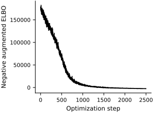
The array above contains the posterior means of the five candidate particles. Some should remain near the three true particles, while the unnecessary ones should move away or become diffuse.

fig = plt.figure(
    figsize=FIGURE_SIZES["full_standard"], constrained_layout=True
)
ax = fig.add_subplot(111, projection="3d")
ax.scatter(
    true_positions[:, 0],
    true_positions[:, 1],
    true_positions[:, 2],
    marker="o",
    facecolors="none",
    edgecolors="black",
    linewidths=1.2,
    depthshade=False,
    s=90,
    label="True particles",
)
ax.scatter(
    mu[:, 0],
    mu[:, 1],
    mu[:, 2],
    marker="^",
    facecolors="0.55",
    edgecolors="black",
    s=40,
    linewidths=0.9,
    depthshade=False,
    label="Candidate means",
)

for idx in range(num_candidate_particles):
    ax.text(mu[idx, 0], mu[idx, 1], mu[idx, 2], f"  c{idx + 1}", fontsize=8)

ax.set_xlabel("$x$")
ax.set_ylabel("$y$")
ax.set_zlabel("$z$", labelpad=-5)
ax.legend(loc="upper left")
finalize_axes(keep_box=False)
plt.show()

candidate_summary = {
    f"candidate_{idx + 1}": {
        "mean": mu[idx],
        "std": std[idx],
        "radius": float(jnp.linalg.norm(mu[idx])),
    }
    for idx in range(num_candidate_particles)
}
candidate_summary

{'candidate_1': {'mean': Array([-0.55077836, -0.20136227,  0.25287222], dtype=float64),
  'std': Array([0.01490007, 0.01105111, 0.01535589], dtype=float64),
  'radius': 0.6386297279072398},
 'candidate_2': {'mean': Array([-1.74078498, -0.08135893, -1.05533435], dtype=float64),
  'std': Array([0.1872365 , 0.22821919, 0.25865313], dtype=float64),
  'radius': 2.037322311779673},
 'candidate_3': {'mean': Array([0.4491913 , 0.0991566 , 0.20150746], dtype=float64),
  'std': Array([0.01360029, 0.01068519, 0.01490371], dtype=float64),
  'radius': 0.5022052450909544},
 'candidate_4': {'mean': Array([-0.04902262,  0.44876755, -0.34782105], dtype=float64),
  'std': Array([0.01215099, 0.01122402, 0.01445432], dtype=float64),
  'radius': 0.5698903525058933},
 'candidate_5': {'mean': Array([-1.58487621, -1.2124272 , -1.08453771], dtype=float64),
  'std': Array([0.1432076 , 0.40274884, 0.24300746], dtype=float64),
  'radius': 2.2711306384619103}}

Post-processing: identify the reconstructed particles

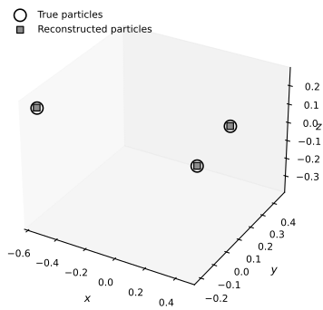
The variational posterior is defined over an overcomplete set of candidates, so we still need a simple rule for deciding which candidates represent distinct particles. We use two heuristics:

1. Ignore candidates that have drifted too far from the imaging volume.

2. Cluster candidates that are closer than a small distance threshold.

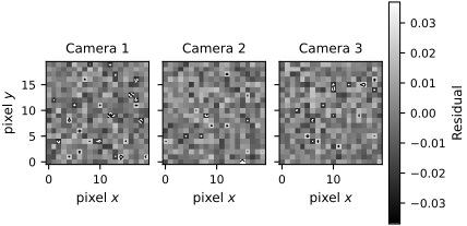
This post-processing turns the overcomplete representation into a sparse reconstructed point cloud. In the stored run, it recovers all three true particles with no extra detected particles; the root mean square coordinate error under the best matching assignment is \(0.0015\) in the example’s coordinate units.

def cluster_active_particles(candidate_positions, candidate_std, radius_threshold=1.6, merge_threshold=0.18):
    scores = jnp.linalg.norm(candidate_std, axis=1)
    active_particles = []

    for idx in map(int, jnp.argsort(scores)):
        point = candidate_positions[idx]
        if float(jnp.linalg.norm(point)) > radius_threshold:
            continue
        if any(float(jnp.linalg.norm(point - q)) < merge_threshold for q in active_particles):
            continue
        active_particles.append(point)

    if not active_particles:
        return jnp.empty((0, 3), dtype=jnp.float64)
    return jnp.stack(active_particles)


def best_rms_error(reconstructed, reference):
    if reconstructed.shape[0] < reference.shape[0]:
        return jnp.inf, None

    best_error = jnp.inf
    best_subset = None
    reference_indices = tuple(range(reference.shape[0]))
    for subset in itertools.combinations(range(reconstructed.shape[0]), reference.shape[0]):
        subset_points = reconstructed[jnp.array(subset)]
        for perm in itertools.permutations(reference_indices):
            candidate = subset_points[jnp.array(perm)]
            error = jnp.sqrt(jnp.mean((candidate - reference) ** 2))
            if error < best_error:
                best_error = error
                best_subset = candidate
    return best_error, best_subset


reconstructed_particles = cluster_active_particles(mu, std)
rms_error, matched_particles = best_rms_error(reconstructed_particles, true_positions)

fig = plt.figure(
    figsize=FIGURE_SIZES["full_standard"], constrained_layout=True
)
ax = fig.add_subplot(111, projection="3d")
ax.scatter(
    true_positions[:, 0],
    true_positions[:, 1],
    true_positions[:, 2],
    marker="o",
    facecolors="none",
    edgecolors="black",
    linewidths=1.2,
    depthshade=False,
    s=100,
    label="True particles",
)
if reconstructed_particles.shape[0] > 0:
    ax.scatter(
        reconstructed_particles[:, 0],
        reconstructed_particles[:, 1],
        reconstructed_particles[:, 2],
        marker="s",
        facecolors="0.55",
        edgecolors="black",
        linewidths=0.9,
        depthshade=False,
        s=30,
        label="Reconstructed particles",
    )
ax.set_xlabel("$x$")
ax.set_ylabel("$y$")
ax.set_zlabel("$z$", labelpad=-5)
ax.legend(loc="upper left")
finalize_axes(keep_box=False)
plt.show()

num_detected = int(reconstructed_particles.shape[0])
num_true = int(true_positions.shape[0])
num_matches = min(num_detected, num_true)
ghost_fraction = max(num_detected - num_true, 0) / max(num_detected, 1)

Markdown(
    f"""
**Reconstruction summary**

- True particles: `{num_true}`
- Reconstructed particles after clustering: `{num_detected}`
- RMS coordinate error against the best matching assignment: `{float(rms_error):.4f}`
- Ghost fraction after clustering: `{ghost_fraction:.3f}`
"""
)

Reconstruction summary

• True particles: 3

• Reconstructed particles after clustering: 3

• RMS coordinate error against the best matching assignment: 0.0015

• Ghost fraction after clustering: 0.000

fig, axes = plt.subplots(
    1,
    3,
    figsize=FIGURE_SIZES["full_landscape"],
    sharex=True,
    sharey=True,
    constrained_layout=True,
)
reconstructed_image = render_all_cameras(reconstructed_particles)
residual_images = observed_images - reconstructed_image
residual_limit = float(jnp.max(jnp.abs(residual_images)))
residual_norm = mpl.colors.TwoSlopeNorm(
    vmin=-residual_limit, vcenter=0.0, vmax=residual_limit
)
contour_level = 2.0 * noise_std

for idx, ax in enumerate(axes):
    difference = residual_images[idx]
    image = ax.imshow(
        difference,
        origin="lower",
        cmap="gray",
        norm=residual_norm,
        interpolation="nearest",
    )
    ax.contour(
        difference,
        levels=[-contour_level],
        colors="white",
        linestyles="--",
        linewidths=0.7,
    )
    ax.contour(
        difference,
        levels=[contour_level],
        colors="black",
        linestyles="-",
        linewidths=0.7,
    )
    ax.set_title(f"Camera {idx + 1}")
    ax.set_xlabel("pixel $x$")
axes[0].set_ylabel("pixel $y$")
colorbar = fig.colorbar(image, ax=axes, fraction=0.035, pad=0.02)
colorbar.set_label("Residual")
finalize_axes(axes, keep_box=True)
plt.show()

Discussion

Stochastic volumetric reconstruction combines a differentiable camera model, a probabilistic model for the unknown particle locations, and a variational approximation of the posterior. The overcomplete candidate set lets optimization suppress unnecessary particles. This small example turns the combinatorial reconstruction problem into continuous optimization over a probabilistic model.