Random-walk Metropolis with BlackJAX

The preceding section derived the Metropolis–Hastings transition and the diagnostics needed to assess a finite run. This notebook implements a Gaussian random-walk kernel with BlackJAX (Cabezas et al., 2024). The example separates warmup from inference, retains every inference draw, and checks the computation against properties of the target that are known exactly.

Banana-shaped target

Let

\[\begin{split} U= \begin{bmatrix}U_1\\U_2\end{bmatrix} \sim \mathcal{N}\!\left( 0, \Sigma_\rho \right), \qquad \Sigma_\rho= \begin{bmatrix} 1 & \rho\\ \rho & 1 \end{bmatrix}, \end{split}\]

and define

\[ X_1=aU_1, \qquad X_2=\frac{U_2}{a}+b\left(U_1^2+a^2\right). \]

Write \(X=(X_1,X_2)^{\mathsf T}\in\mathbb{R}^2\) and let \(x=(x_1,x_2)^{\mathsf T}\in\mathbb{R}^2\) denote one of its realizations. We use \(a=1.15\), \(b=0.5\), and \(\rho=0.9\), the parameters of the banana-shaped example in Wang et al. (2019). The inverse transformation is

\[ u_1(x)=\frac{x_1}{a}, \qquad u_2(x)=a\left[x_2-b\left(\left(\frac{x_1}{a}\right)^2+a^2\right)\right]. \]

Its Jacobian determinant is one because

\[\begin{split} \det \begin{bmatrix} \partial u_1/\partial x_1 & \partial u_1/\partial x_2\\ \partial u_2/\partial x_1 & \partial u_2/\partial x_2 \end{bmatrix} = \det \begin{bmatrix} a^{-1} & 0\\ -2bx_1/a & a \end{bmatrix} =1. \end{split}\]

Therefore the normalized target density is \(\pi(x)=\phi_{\Sigma_\rho}(u(x))\), where \(\phi_{\Sigma_\rho}\) is the centered Gaussian density with covariance \(\Sigma_\rho\).

a = 1.15
b = 0.5
rho = 0.9
correlation = jnp.array([[1.0, rho], [rho, 1.0]])


def banana_logdensity(x):
    # Log density induced by the unit-Jacobian banana transformation.
    x1, x2 = x
    u1 = x1 / a
    u2 = a * (x2 - b * (u1**2 + a**2))
    u = jnp.array([u1, u2])
    return multivariate_normal.logpdf(u, jnp.zeros(2), correlation)


grid_x = jnp.linspace(-4.0, 4.0, 160)
grid_y = jnp.linspace(-2.0, 7.0, 180)
X_grid, Y_grid = jnp.meshgrid(grid_x, grid_y)
grid_points = jnp.stack([X_grid.ravel(), Y_grid.ravel()], axis=1)
target_density = jnp.exp(vmap(banana_logdensity)(grid_points)).reshape(X_grid.shape)


def draw_target_contours(ax):
    maximum = float(jnp.max(target_density))
    levels = np.linspace(0.04 * maximum, 0.92 * maximum, 9)
    ax.contour(
        np.asarray(X_grid),
        np.asarray(Y_grid),
        np.asarray(target_density),
        levels=levels,
        colors="0.35",
        linewidths=0.8,
    )
    ax.set_xlim(-4.0, 4.0)
    ax.set_ylim(-2.0, 7.0)
    ax.set_aspect("equal")
    ax.set_xlabel(r"$x_1$")
    ax.set_ylabel(r"$x_2$")
    finish_axes(ax, boxed=True)
    return ax


fig, ax = plt.subplots(figsize=FIGURE_SIZES["half_tall"], constrained_layout=True)
draw_target_contours(ax)
ax.set_title("Banana-shaped target density");

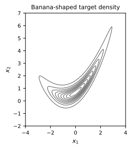
Fig. 7 Contours of the banana-shaped target density for \(a=1.15\), \(b=0.5\), and \(\rho=0.9\).

Gaussian random-walk kernel

At state \(x\), the proposal is

\[ X'=x+\varepsilon, \qquad \varepsilon\sim\mathcal{N}(0,\sigma^2I_2). \]

Here \(\sigma>0\) is the proposal scale and \(I_2\) is the \(2\times2\) identity matrix.

Thus \(q(x'\mid x)=q(x\mid x')\), and the proposal-density ratio cancels from the Metropolis–Hastings acceptance probability:

\[ \alpha(x,x') = \min\!\left\{1,\frac{\pi(x')}{\pi(x)}\right\}. \]

We fix \(\sigma=0.7\) before collecting inference draws. This value is suitable for the demonstration; in an application it should be selected in a separate pilot or warmup calculation rather than tuned using retained inference draws.

proposal_scale = 0.7

kernel = blackjax.additive_step_random_walk.normal_random_walk(
    banana_logdensity,
    proposal_scale * jnp.ones(2),
)


def scan_step(carry, _):
    key, state = carry
    key, transition_key = jrandom.split(key)
    next_state, info = kernel.step(transition_key, state)
    output = (next_state.position, info.is_accepted)
    return (key, next_state), output


def run_chain(key, initial_state, num_steps):
    (_, final_state), output = lax.scan(
        scan_step,
        (key, initial_state),
        None,
        length=num_steps,
    )
    positions, is_accepted = output
    return final_state, positions, is_accepted


def demo_scan_step(carry, _):
    key, state = carry
    key, transition_key = jrandom.split(key)
    proposal_key, _ = jrandom.split(transition_key)
    candidate = state.position + proposal_scale * jrandom.normal(
        proposal_key,
        shape=state.position.shape,
    )
    next_state, info = kernel.step(transition_key, state)
    output = (next_state.position, info.is_accepted, candidate)
    return (key, next_state), output


def run_demo(key, initial_state, num_steps):
    (_, final_state), output = lax.scan(
        demo_scan_step,
        (key, initial_state),
        None,
        length=num_steps,
    )
    positions, is_accepted, candidates = output
    return final_state, positions, is_accepted, candidates


master_key = jrandom.PRNGKey(20260919)
demo_key, warmup_key, inference_key = jrandom.split(master_key, 3)

The next figure makes rejection visible. A filled circle marks an accepted candidate. A cross marks a rejected candidate; after rejection, the state is repeated.

demo_initial_position = jnp.array([3.0, 5.0])
_, demo_states, demo_accept, demo_proposals = run_demo(
    demo_key,
    kernel.init(demo_initial_position),
    14,
)

demo_previous = np.vstack(
    [np.asarray(demo_initial_position), np.asarray(demo_states[:-1])]
)

fig, ax = plt.subplots(figsize=FIGURE_SIZES["full_standard"], constrained_layout=True)
draw_target_contours(ax)
ax.set_xlim(-4.0, 4.6)
ax.plot(
    demo_initial_position[0],
    demo_initial_position[1],
    marker="*",
    color="black",
    markersize=8,
    linestyle="none",
    label="initial state",
)

accepted_label_used = False
rejected_label_used = False
for previous, proposal, accepted in zip(
    demo_previous,
    np.asarray(demo_proposals),
    np.asarray(demo_accept),
):
    if accepted:
        ax.annotate(
            "",
            xy=proposal,
            xytext=previous,
            arrowprops={"arrowstyle": "->", "color": "0.10", "linewidth": 0.9},
        )
        ax.plot(
            proposal[0],
            proposal[1],
            marker="o",
            markerfacecolor="black",
            markeredgecolor="black",
            markersize=3.5,
            linestyle="none",
            label="accepted candidate" if not accepted_label_used else None,
        )
        accepted_label_used = True
    else:
        ax.annotate(
            "",
            xy=proposal,
            xytext=previous,
            arrowprops={
                "arrowstyle": "->",
                "color": "0.60",
                "linewidth": 0.8,
                "linestyle": ":",
            },
        )
        ax.plot(
            proposal[0],
            proposal[1],
            marker="x",
            color="0.45",
            markersize=5,
            linestyle="none",
            label="rejected candidate" if not rejected_label_used else None,
        )
        rejected_label_used = True

ax.legend(loc="upper left")
ax.set_title("Fourteen random-walk proposals");

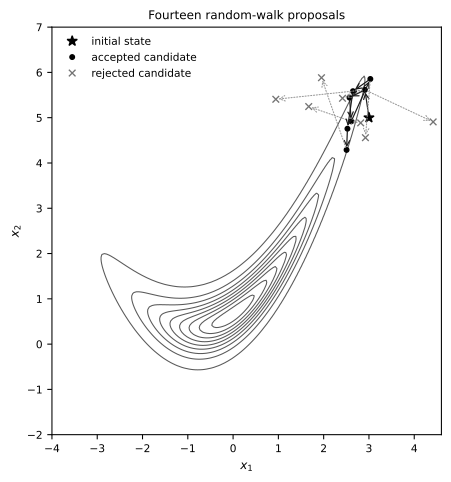
Fig. 8 Accepted and rejected candidates from fourteen random-walk Metropolis transitions. A rejection leaves the chain state unchanged.

Warmup and inference draws

We run four chains from dispersed initial positions. The first \(3{,}000\) iterations form a pre-specified warmup phase used only to reduce sensitivity to the initial positions. The kernel has no adaptive parameter in this example. We then start a separate inference phase from the four warmup endpoints and retain all \(40{,}000\) draws from each chain.

The warmup length is not inferred from a retrospective threshold crossing. Instead, the post-warmup draws are assessed using multiple-chain plots and diagnostics.

initial_positions = jnp.array(
    [
        [-4.0, 1.0],
        [-1.0, -1.0],
        [1.0, 4.0],
        [4.0, 6.0],
    ]
)

num_chains = initial_positions.shape[0]
num_warmup = 3_000
num_draws = 40_000

warmup_keys = jrandom.split(warmup_key, num_chains)
initial_states = vmap(kernel.init)(initial_positions)
warmup_final_states, warmup_samples, warmup_accepted = vmap(
    run_chain,
    in_axes=(0, 0, None),
)(warmup_keys, initial_states, num_warmup)

inference_keys = jrandom.split(inference_key, num_chains)
_, samples, inference_accepted = vmap(
    run_chain,
    in_axes=(0, 0, None),
)(inference_keys, warmup_final_states, num_draws)

samples.shape

(4, 40000, 2)

The trace display includes the entire warmup and the first \(2{,}000\) inference draws. The vertical line marks the boundary; all numerical diagnostics below use the complete inference phase.

trace_draws = 2_000
trace_values = np.concatenate(
    [np.asarray(warmup_samples), np.asarray(samples[:, :trace_draws])],
    axis=1,
)
trace_iteration = np.arange(-num_warmup + 1, trace_draws + 1)

fig, axes = plt.subplots(
    2,
    1,
    sharex=True,
    figsize=FIGURE_SIZES["full_standard"],
    constrained_layout=True,
)
for chain in range(num_chains):
    color, linestyle = CHAIN_STYLES[chain]
    for coordinate, ax in enumerate(axes):
        ax.plot(
            trace_iteration,
            trace_values[chain, :, coordinate],
            color=color,
            linestyle=linestyle,
            linewidth=0.55,
            rasterized=True,
            label=f"chain {chain + 1}" if coordinate == 0 else None,
        )

for coordinate, ax in enumerate(axes):
    ax.axvline(0, color="black", linewidth=0.9)
    ax.set_ylabel(fr"$x_{coordinate + 1}$")
axes[0].legend(ncol=4, loc="upper center")
axes[-1].set_xlabel("Iteration relative to the end of warmup")
finish_axes(axes);

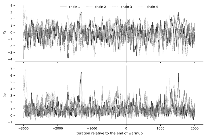
Fig. 9 Warmup and initial inference traces for four dispersed chains. The vertical line marks the end of warmup.

Multiple-chain diagnostics

We compute the rank-normalized split and folded \(\widehat R\), together with bulk and tail effective sample sizes, on the post-warmup draws (Vehtari et al., 2021). The acceptance rate describes the kernel’s local behavior but does not establish convergence by itself.

rhat = np.asarray(blackjax.rhat(samples))
bulk_ess = np.asarray(blackjax.ess_bulk(samples))
tail_ess = np.asarray(blackjax.ess_tail(samples))
acceptance_rate = np.asarray(inference_accepted).mean(axis=1)

diagnostic_rows = [
    ["Rank-normalized split/folded R-hat", f"{rhat[0]:.4f}", f"{rhat[1]:.4f}"],
    ["Bulk ESS", f"{bulk_ess[0]:.0f}", f"{bulk_ess[1]:.0f}"],
    ["Tail ESS", f"{tail_ess[0]:.0f}", f"{tail_ess[1]:.0f}"],
]
diagnostic_latex = rf'''
\begin{{tabular}}{{lrr}}
\hline
Quantity & $x_1$ & $x_2$ \\
\hline
Rank-normalized split/folded $\widehat R$ & {rhat[0]:.4f} & {rhat[1]:.4f} \\
Bulk ESS & {bulk_ess[0]:.0f} & {bulk_ess[1]:.0f} \\
Tail ESS & {tail_ess[0]:.0f} & {tail_ess[1]:.0f} \\
\hline
\end{{tabular}}
'''
math_class = 'class="math notranslate nohighlight"'
diagnostic_html_headers = [
    "Quantity",
    f"<span {math_class}>\\(x_1\\)</span>",
    f"<span {math_class}>\\(x_2\\)</span>",
]
diagnostic_html_rows = [
    [
        f"Rank-normalized split/folded <span {math_class}>\\(\\widehat R\\)</span>",
        diagnostic_rows[0][1],
        diagnostic_rows[0][2],
    ],
    diagnostic_rows[1],
    diagnostic_rows[2],
]
display_book_table(
    ["Quantity", "x1", "x2"],
    diagnostic_rows,
    diagnostic_latex,
    html_headers=diagnostic_html_headers,
    html_rows=diagnostic_html_rows,
)
print(
    "Per-chain acceptance rates: "
    + ", ".join(f"{rate:.3f}" for rate in acceptance_rate)
)

Quantity	\(x_1\)	\(x_2\)
Rank-normalized split/folded \(\widehat R\)	1.0005	1.0006
Bulk ESS	2612	3012
Tail ESS	2061	2139

Per-chain acceptance rates: 0.402, 0.399, 0.401, 0.401

Rank histograms provide a complementary graphical check. If the chains explore the same distribution, each chain should contribute comparably throughout the pooled ranks. Exact uniformity is neither expected nor required.

num_rank_bins = 20
fig, axes = plt.subplots(
    1,
    2,
    figsize=FIGURE_SIZES["full_standard"],
    constrained_layout=True,
)

for coordinate, ax in enumerate(axes):
    pooled = np.asarray(samples[:, :, coordinate])
    ranks = rankdata(pooled.ravel(), method="average").reshape(pooled.shape)
    bin_edges = np.linspace(0.5, ranks.size + 0.5, num_rank_bins + 1)
    bin_centers = 0.5 * (bin_edges[:-1] + bin_edges[1:])
    for chain in range(num_chains):
        color, linestyle = CHAIN_STYLES[chain]
        counts, _ = np.histogram(ranks[chain], bins=bin_edges)
        ax.step(
            bin_centers,
            counts,
            where="mid",
            color=color,
            linestyle=linestyle,
            label=f"chain {chain + 1}",
        )
    ax.axhline(num_draws / num_rank_bins, color="0.75", linewidth=0.8)
    ax.set_title(fr"Ranks for $x_{coordinate + 1}$")
    ax.set_xlabel("Pooled rank")
    ax.set_ylabel("Count")

axes[0].legend(ncol=2)
finish_axes(axes);

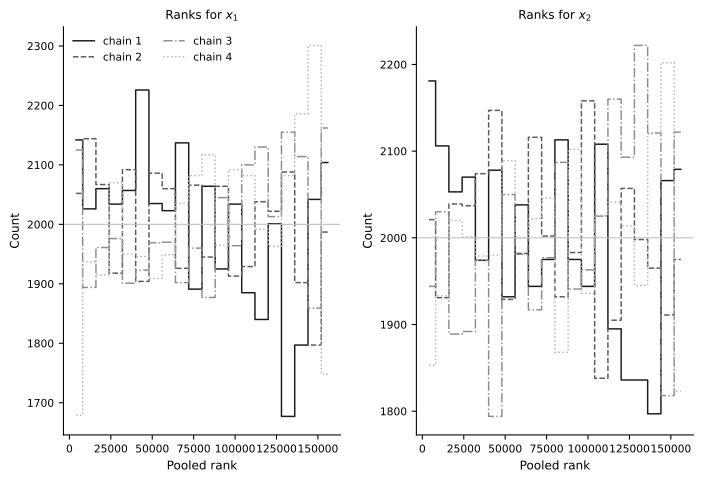
Fig. 10 Pooled-rank histograms for the four inference chains. Comparable contributions across ranks support, but do not prove, chain agreement.

Monte Carlo precision and an exact check

The transformation gives several exact moments:

\[\begin{split} \begin{aligned} \mathbb{E}[X_1]&=0, &\mathbb{E}[X_2]&=b(1+a^2),\\ \mathbb{E}[X_1^2]&=a^2, &\mathbb{E}[X_1X_2]&=\rho,\\ \operatorname{Var}(X_2)&=a^{-2}+2b^2. \end{aligned} \end{split}\]

The last identity uses \(\operatorname{Cov}(U_2,U_1^2)=0\), since every centered third-order Gaussian moment vanishes. Hence

\[ \mathbb{E}[X_2^2] = a^{-2}+2b^2+b^2(1+a^2)^2. \]

For each moment \(g(X)\), the table estimates

\[ \operatorname{MCSE}(\bar g) \approx \sqrt{\frac{\widehat{\operatorname{Var}}(g(X))}{N_{\mathrm{eff},g}}}. \]

Here \(\bar g\) is the average of \(g(X)\) over all retained chains and draws, \(\widehat{\operatorname{Var}}(g(X))\) is their pooled sample variance, and \(N_{\mathrm{eff},g}\) is the estimand-specific effective sample size for that average.

moment_draws = jnp.stack(
    [
        samples[..., 0],
        samples[..., 1],
        samples[..., 0] ** 2,
        samples[..., 0] * samples[..., 1],
        samples[..., 1] ** 2,
    ],
    axis=-1,
)

exact_moments = np.array(
    [
        0.0,
        b * (1.0 + a**2),
        a**2,
        rho,
        a ** (-2) + 2.0 * b**2 + b**2 * (1.0 + a**2) ** 2,
    ]
)
moment_names = [
    "E[X1]",
    "E[X2]",
    "E[X1^2]",
    "E[X1 X2]",
    "E[X2^2]",
]
moment_names_latex = [
    r"$\mathbb{E}[X_1]$",
    r"$\mathbb{E}[X_2]$",
    r"$\mathbb{E}[X_1^2]$",
    r"$\mathbb{E}[X_1X_2]$",
    r"$\mathbb{E}[X_2^2]$",
]
moment_names_html = [
    f"<span {math_class}>\\(\\mathbb{{E}}[X_1]\\)</span>",
    f"<span {math_class}>\\(\\mathbb{{E}}[X_2]\\)</span>",
    f"<span {math_class}>\\(\\mathbb{{E}}[X_1^2]\\)</span>",
    f"<span {math_class}>\\(\\mathbb{{E}}[X_1X_2]\\)</span>",
    f"<span {math_class}>\\(\\mathbb{{E}}[X_2^2]\\)</span>",
]

moment_estimates = np.asarray(moment_draws.mean(axis=(0, 1)))
moment_ess = np.asarray(blackjax.ess(moment_draws))
moment_rhat = np.asarray(blackjax.rhat(moment_draws))
moment_variances = np.asarray(moment_draws).reshape(-1, len(moment_names)).var(
    axis=0,
    ddof=1,
)
moment_mcse = np.sqrt(moment_variances / moment_ess)

moment_rows = []
for name, exact, estimate, mcse, value_rhat, value_ess in zip(
    moment_names,
    exact_moments,
    moment_estimates,
    moment_mcse,
    moment_rhat,
    moment_ess,
):
    moment_rows.append(
        [
            name,
            f"{exact:.4f}",
            f"{estimate:.4f}",
            f"{mcse:.4f}",
            f"{value_rhat:.4f}",
            f"{value_ess:.0f}",
        ]
    )

moment_latex_rows = []
for name, row in zip(moment_names_latex, moment_rows):
    moment_latex_rows.append(name + " & " + " & ".join(row[1:]) + r" \\")
moment_latex = r'''
\begin{tabular}{lrrrrr}
\hline
Estimand & Exact & Estimate & MCSE & $\widehat R$ & ESS for $\bar g$ \\
\hline
''' + "\n".join(moment_latex_rows) + r'''
\hline
\end{tabular}
'''
moment_html_rows = [
    [html_name] + row[1:]
    for html_name, row in zip(moment_names_html, moment_rows)
]
display_book_table(
    ["Estimand", "Exact", "Estimate", "MCSE", "R-hat", "ESS for mean"],
    moment_rows,
    moment_latex,
    html_headers=[
        "Estimand",
        "Exact",
        "Estimate",
        "MCSE",
        f"<span {math_class}>\\(\\widehat R\\)</span>",
        f"ESS for <span {math_class}>\\(\\bar g\\)</span>",
    ],
    html_rows=moment_html_rows,
)

Estimand	Exact	Estimate	MCSE	\(\widehat R\)	ESS for \(\bar g\)
\(\mathbb{E}[X_1]\)	0.0000	-0.0195	0.0221	1.0005	2651
\(\mathbb{E}[X_2]\)	1.1612	1.1392	0.0243	1.0006	1928
\(\mathbb{E}[X_1^2]\)	1.3225	1.2931	0.0335	1.0004	2895
\(\mathbb{E}[X_1X_2]\)	0.9000	0.8028	0.0714	1.0006	1609
\(\mathbb{E}[X_2^2]\)	2.6046	2.4318	0.1275	1.0007	1491

Every post-warmup state remains in these calculations. Correlation lowers effective sample size, but ESS does not define a thinning interval. Routine thinning would discard information; it is appropriate only when storage or downstream processing is the binding constraint (Link and Eaton, 2012).

For a readable final plot, the code below displays every fortieth draw. This display reduction is not analytic thinning: all numerical summaries and moment estimates above use the complete array of \(4\times40{,}000\) inference draws.

display_stride = 40
display_samples = np.asarray(samples[:, ::display_stride]).reshape(-1, 2)

fig, ax = plt.subplots(figsize=FIGURE_SIZES["full_standard"], constrained_layout=True)
draw_target_contours(ax)
ax.scatter(
    display_samples[:, 0],
    display_samples[:, 1],
    s=5,
    facecolors="none",
    edgecolors="0.10",
    linewidths=0.35,
    alpha=0.35,
    rasterized=True,
)
ax.set_title("Displayed inference draws and target contours");

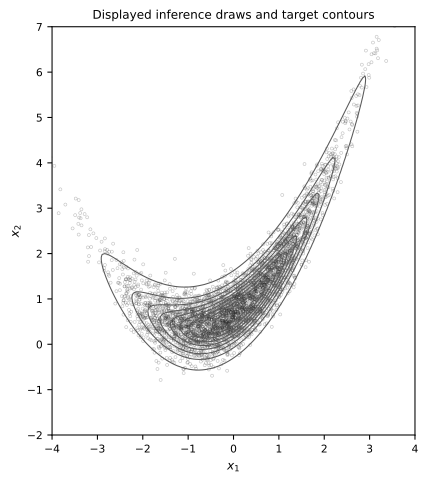
Fig. 11 A display subset of inference draws over the target-density contours. Numerical summaries use all retained draws.

Diagnostic interpretation

For this stored run, the coordinate and moment \(\widehat R\) values satisfy the \(1.01\) warning screen, the rank plots show no clear chain separation, and the exact moments agree with the Monte Carlo estimates at the scale indicated by their MCSEs. These checks reveal no evident failure for the displayed quantities, but no finite diagnostic certifies convergence.

The effective sample sizes are nevertheless a small fraction of the \(160{,}000\) retained states. The curved target forces an isotropic random walk to explore through many local moves. The next notebook uses gradients and Hamiltonian dynamics to make proposals that travel farther along this geometry.

Exercises

1. Use a separate pilot run to compare several values of proposal_scale. Fix the selected value, generate fresh inference draws, and compare acceptance rate, \(\widehat R\), bulk and tail ESS, and MCSE. Explain why acceptance rate alone is insufficient.

2. Move the four initial positions farther into the tails. Keep the warmup length fixed and assess whether the post-warmup chains still explore the same distribution. Use both trace and rank plots.

3. Construct an independent Metropolis–Hastings kernel with blackjax.irmh. Define one callable that draws \(X'\sim q\) and another that evaluates \(\log q(x')\) so that BlackJAX can include the Hastings correction. Compare a proposal with broad target coverage to one with poor overlap. If \(q(x')=0\) on a region where \(\pi(x')>0\), explain why the kernel is not \(\pi\)-irreducible, meaning that the chain cannot reach every region to which \(\pi\) assigns positive probability from every starting state, and why invariance alone does not ensure convergence to \(\pi\) from an arbitrary initial state.