Polynomial Chaos for a Uniform Input

A polynomial-chaos approximation expands a random model response in orthonormal polynomials matched to the input distribution. The simplest continuous case is a uniform random variable \(\Xi\sim\mathcal{U}[0,1]\), whose probability density is one on \([0,1]\). We work in the Hilbert space

\[ L^2(\Xi)=\left\{f:[0,1]\to\mathbb{R}:\mathbb{E}[f(\Xi)^2]<\infty\right\}, \]

where functions that agree almost everywhere are identified. The inner product and norm are

\[ \langle f,g\rangle=\mathbb{E}[f(\Xi)g(\Xi)] =\int_0^1 f(\xi)g(\xi)\,d\xi, \qquad \|f\|=\sqrt{\langle f,f\rangle}. \]

The probability density is part of the construction: a different input distribution produces a different inner product and therefore a different polynomial basis.

xi = sp.symbols("xi", real=True)


def inner_product(f, g):
    return sp.integrate(f * g, (xi, 0, 1))


def norm(f):
    return sp.sqrt(inner_product(f, f))

Gram–Schmidt construction

Let \(p_n(\xi)=\xi^n\) for \(n=0,1,\ldots\). The monomials are linearly independent, and Gram–Schmidt converts them into orthonormal polynomials. Once \(\phi_0,\ldots,\phi_{n-1}\) have been constructed, define

\[ \widetilde{\phi}_n =p_n-\sum_{k=0}^{n-1}\langle p_n,\phi_k\rangle\phi_k, \qquad \phi_n=\frac{\widetilde{\phi}_n}{\|\widetilde{\phi}_n\|}. \]

The sum is empty when \(n=0\). The first three polynomials are

\[ \phi_0(\xi)=1, \qquad \phi_1(\xi)=\sqrt{3}(2\xi-1), \qquad \phi_2(\xi)=\sqrt{5}(6\xi^2-6\xi+1). \]

def gram_schmidt(polynomials):
    orthonormal_polynomials = []
    for polynomial in polynomials:
        residual = polynomial
        for phi in orthonormal_polynomials:
            residual -= inner_product(polynomial, phi) * phi
        orthonormal_polynomials.append(sp.factor(residual / norm(residual)))
    return orthonormal_polynomials


degree = 5
monomials = [xi ** n for n in range(degree + 1)]
basis_polynomials = gram_schmidt(monomials)

Shifted Legendre form

Let \(P_n\) be the degree-\(n\) Legendre polynomial on \([-1,1]\), normalized by \(P_n(1)=1\). The change of variable \(z=2\xi-1\) gives the closed form

\[ \phi_n(\xi)=\sqrt{2n+1}\,P_n(2\xi-1), \qquad n=0,1,\ldots, \]

and hence

\[ \int_0^1\phi_n(\xi)\phi_m(\xi)\,d\xi=\delta_{nm}, \]

where \(\delta_{nm}\) is one when \(n=m\) and zero otherwise. The complete sequence is an orthonormal basis of \(L^2(\Xi)\), while \(\phi_0,\ldots,\phi_p\) span the polynomials of degree at most \(p\). These are the shifted, normalized Legendre polynomials used for a uniform polynomial-chaos expansion (Xiu and Karniadakis, 2002).

legendre_basis = [
    sp.sqrt(2 * n + 1) * sp.legendre(n, 2 * xi - 1)
    for n in range(degree + 1)
]

for phi_gram_schmidt, phi_legendre in zip(basis_polynomials, legendre_basis):
    assert sp.simplify(phi_gram_schmidt - phi_legendre) == 0

The Gram matrix \(G\) has entries \(G_{nm}=\langle\phi_n,\phi_m\rangle\). Exact symbolic integration returns the \(6\times6\) identity matrix.

gram_matrix = sp.Matrix(
    [
        [sp.simplify(inner_product(phi_n, phi_m)) for phi_m in basis_polynomials]
        for phi_n in basis_polynomials
    ]
)
assert gram_matrix == sp.eye(degree + 1)
gram_matrix

\[\begin{split}\displaystyle \left[\begin{matrix}1 & 0 & 0 & 0 & 0 & 0\\0 & 1 & 0 & 0 & 0 & 0\\0 & 0 & 1 & 0 & 0 & 0\\0 & 0 & 0 & 1 & 0 & 0\\0 & 0 & 0 & 0 & 1 & 0\\0 & 0 & 0 & 0 & 0 & 1\end{matrix}\right]\end{split}\]

Projection and moments

Let \(f\in L^2(\Xi)\) and let \(Y=f(\Xi)\). For a nonnegative integer \(p\), the degree-\(p\) polynomial-chaos approximation is the orthogonal projection

\[ (\Pi_p f)(\xi)=\sum_{n=0}^{p}c_n\phi_n(\xi), \qquad c_n=\langle f,\phi_n\rangle =\int_0^1f(\xi)\phi_n(\xi)\,d\xi. \]

Because \(\phi_0=1\) and \(\mathbb{E}[\phi_n(\Xi)]=0\) for \(n\geq1\), orthonormality gives

\[ \mathbb{E}[(\Pi_p f)(\Xi)]=c_0=\mathbb{E}[Y], \qquad \operatorname{Var}[(\Pi_p f)(\Xi)]=\sum_{n=1}^{p}c_n^2. \]

For the complete expansion, Parseval’s identity gives \(\operatorname{Var}[Y]=\sum_{n=1}^{\infty}c_n^2\). For a basis \(\{\psi_n\}\) that is orthogonal but not normalized, the coefficient is \(\langle f,\psi_n\rangle/\|\psi_n\|^2\) and its variance contribution is the squared coefficient multiplied by \(\|\psi_n\|^2\).

f_expression = sp.exp(xi)
coefficients = [
    sp.simplify(inner_product(f_expression, phi))
    for phi in basis_polynomials
]
projection_expression = sp.expand(
    sum(
        (coefficient * phi for coefficient, phi in zip(coefficients, basis_polynomials)),
        sp.Integer(0),
    )
)

projection_mean = coefficients[0]
projection_variance = sp.simplify(sum(c ** 2 for c in coefficients[1:]))
exact_mean = inner_product(f_expression, sp.Integer(1))
exact_variance = sp.simplify(inner_product(f_expression - exact_mean, f_expression - exact_mean))
projection_error = sp.sqrt(
    inner_product(f_expression - projection_expression, f_expression - projection_expression)
)

For \(f(\xi)=e^\xi\) and \(p=5\), the following values compare the projected and exact moments. The \(L^2(\Xi)\) error measures the discrepancy between the function and its projection over the entire input distribution.

def numeric_value(expression):
    return float(sp.N(expression, 12))


print(f"projection mean:     {numeric_value(projection_mean):.10f}")
print(f"exact mean:          {numeric_value(exact_mean):.10f}")
print(f"projection variance: {numeric_value(projection_variance):.10f}")
print(f"exact variance:      {numeric_value(exact_variance):.10f}")
print(f"L2 projection error: {numeric_value(projection_error):.3e}")

projection mean:     1.7182818285
exact mean:          1.7182818285
projection variance: 0.2420356075
exact variance:      0.2420356075
L2 projection error: 6.935e-07

Basis and projection

The first panel shows the six orthonormal basis functions. The second compares \(e^\xi\) with its degree-five projection.

grid = np.linspace(0.0, 1.0, 500)
basis_functions = [sp.lambdify(xi, phi, "numpy") for phi in basis_polynomials]
basis_values = np.column_stack(
    [
        np.broadcast_to(np.asarray(function(grid), dtype=float), grid.shape)
        for function in basis_functions
    ]
)
target_function = sp.lambdify(xi, f_expression, "numpy")
projection_function = sp.lambdify(xi, projection_expression, "numpy")

line_styles = ["-", "--", "-.", ":", (0, (3, 1, 1, 1)), (0, (5, 2))]
fig, axes = new_figure(size="full_tall", nrows=2, ncols=1, sharex=True)

for n, line_style in enumerate(line_styles):
    axes[0].plot(grid, basis_values[:, n], label=rf"$\phi_{n}$", linestyle=line_style)
axes[0].set(ylabel=r"$\phi_n(\xi)$", title="Shifted, normalized Legendre basis")
axes[0].legend(loc="center left", bbox_to_anchor=(1.01, 0.5), frameon=False)

axes[1].plot(grid, target_function(grid), label=r"$f(\xi)=e^\xi$")
axes[1].plot(grid, projection_function(grid), "--", label=r"$(\Pi_5 f)(\xi)$")
axes[1].set(xlabel=r"$\xi$", ylabel="Response", title="Degree-five orthogonal projection")
axes[1].legend(frameon=False)

label_panels(axes, fontweight="bold")
finalize_axes(axes, keep_box=False);

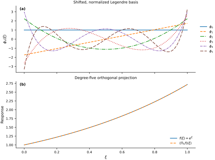
The basis curves are evaluated from exact symbolic expressions in double precision. The degree-five approximation is visually indistinguishable from \(e^\xi\) on this scale, and the \(L^2(\Xi)\) error reported above quantifies the remaining difference. Because these are orthogonal projections onto nested polynomial spaces, increasing the degree cannot increase the \(L^2(\Xi)\) error.

Exercise

Repeat the projection with degrees \(p=0,1,\ldots,5\). Compare the mean, variance, and \(L^2(\Xi)\) error. Explain why every truncation reproduces the exact mean, while the projected variance increases toward the exact variance as additional squared coefficients are included.

Distribution-matched polynomial bases

The orthonormal basis must match the input distribution. Replacing the uniform density with the standard normal density changes the inner product; applying the same construction then produces normalized Hermite polynomials. For higher degrees and more general probability laws, a three-term recurrence is more stable than direct Gram–Schmidt evaluation (Gautschi, 1994).