Bayesian PINNs for Inverse Problems

In the previous section we trained a deterministic inverse PINN and recovered a single best-fit value of the unknown conductivity. The remaining inverse-problem question is the uncertainty in that conductivity and in the reconstructed state.

Bayesian physics-informed neural networks (B-PINNs) address this question by defining a posterior distribution over the unknown quantities rather than returning only one optimizer output. The general framework was introduced by Yang et al. (2021), building directly on the PINN formulation of Raissi et al. (2019).

Bayesian inference for a large neural network can be expensive, so this section uses a deliberately small example. We keep the same one-dimensional diffusion inverse problem and infer the 25 network parameters together with the unknown conductivity. The finite network and statistical model are specified below.

Problem Setup

We again study

\[\begin{split} \begin{aligned} -\theta u''(x) &= \sin(\pi x), \quad x \in (0,1),\\ u(0) &= 0,\\ u(1) &= 0, \end{aligned} \end{split}\]

with unknown conductivity \(\theta > 0\).

The exact solution is still

\[ u^\star(x;\theta) = \frac{\sin(\pi x)}{\theta \pi^2}, \]

and we use it only to manufacture noisy observations. The difference from the previous section is not the PDE. It is the inference target. Instead of searching for a single minimizer of the PINN loss, we will sample from a posterior distribution over the neural-network parameters and \(\theta\). The synthetic observations are shown in Fig. 57.

In B-PINNs the PDE residual supplies additional information through a Gaussian pseudo-likelihood, defined below.

true_theta = 0.7
noise_std = 3e-3
width = 8
n_obs = 9

def source_term(x):
    return jnp.sin(jnp.pi * x)

def exact_solution(x, theta=true_theta):
    return jnp.sin(jnp.pi * x) / (theta * jnp.pi**2)

key = jr.PRNGKey(11)
key, noise_key = jr.split(key)

x_obs = jnp.linspace(0.1, 0.9, n_obs)
y_clean = exact_solution(x_obs)
y_obs = y_clean + noise_std * jr.normal(noise_key, x_obs.shape)
x_phys = jnp.linspace(0.0, 1.0, 17)[1:-1]
xs_plot = jnp.linspace(0.0, 1.0, 200)

fig, ax = new_figure("full_standard")
ax.plot(
    xs_plot, exact_solution(xs_plot), color="black", linestyle="-",
    linewidth=1.5, label="exact solution"
)
ax.scatter(
    x_obs, y_obs, s=24, facecolors="white", edgecolors="black",
    linewidths=0.8, zorder=3, label="noisy observations"
)
ax.set(xlabel=r"$x$", ylabel=r"$u(x)$")
ax.legend(loc="upper right")
finalize_axes(ax)
plt.show()

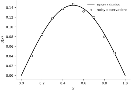
Fig. 57 Synthetic data for the Bayesian inverse problem. The solid curve is the exact solution \(u^\star(x;\theta_{\mathrm{true}})\) for \(\theta_{\mathrm{true}}=0.7\); open circles are the nine observations corrupted by independent Gaussian noise with standard deviation \(3\times 10^{-3}\).

A Small PINN Parameterization

To keep Hamiltonian Monte Carlo affordable, we use a tiny one-hidden-layer network with eight hidden units. As before, the boundary conditions are enforced by construction:

\[ u_\mathbf{w}(x) = x(1-x)\,\text{NN}_\mathbf{w}(x). \]

The conductivity is written as \(\theta = e^{\eta}\) so positivity is automatic. Here the unknowns are the weight vector \(\mathbf{w}\) and the transformed conductivity parameter \(\eta\).

n_nn_params = 3 * width + 1

def unpack(nn_params):
    w1 = nn_params[:width]
    b1 = nn_params[width:2 * width]
    w2 = nn_params[2 * width:3 * width]
    b2 = nn_params[-1]
    return w1, b1, w2, b2

def pinn_solution(x, nn_params):
    w1, b1, w2, b2 = unpack(nn_params)
    hidden = jnp.tanh(w1 * x + b1)
    out = jnp.dot(w2, hidden) + b2
    return x * (1.0 - x) * out

def pinn_residual(x, nn_params, theta):
    u_x = grad(lambda z: pinn_solution(z, nn_params))
    u_xx = grad(u_x)
    return -theta * u_xx(x) - source_term(x)

total_dim = n_nn_params + 1
print(f"Bayesian parameter dimension: {total_dim}")

Bayesian parameter dimension: 26

Deterministic Initialization

Sampling works better when we initialize near a sensible part of parameter space. We therefore minimize the weighted deterministic PINN objective from the previous section and use the result to initialize NUTS. The loss weights of that objective do not match the prior and likelihood scales in the Bayesian model below, so this point is not a maximum a posteriori estimate.

The fitted curve also provides a deterministic reference for the posterior summaries.

def deterministic_loss(params, x_obs, y_obs, x_phys, lambda_data=50.0, lambda_pde=1.0):
    nn_params = params[:-1]
    log_theta = params[-1]
    theta = jnp.exp(log_theta)
    pred_obs = vmap(lambda x: pinn_solution(x, nn_params))(x_obs)
    residual_values = vmap(lambda x: pinn_residual(x, nn_params, theta))(x_phys)
    data_loss = jnp.mean((pred_obs - y_obs) ** 2)
    pde_loss = jnp.mean(residual_values ** 2)
    prior_penalty = 1e-4 * jnp.mean(params ** 2)
    return lambda_data * data_loss + lambda_pde * pde_loss + prior_penalty

key, init_key = jr.split(key)
deterministic_params = jnp.concatenate([
    0.1 * jr.normal(init_key, (n_nn_params,)),
    jnp.array([jnp.log(1.5)]),
])

optimizer = optax.adam(1e-2)
opt_state = optimizer.init(deterministic_params)

@jax.jit
def deterministic_step(params, opt_state):
    loss_value, grads = jax.value_and_grad(deterministic_loss)(params, x_obs, y_obs, x_phys)
    updates, opt_state = optimizer.update(grads, opt_state, params)
    params = optax.apply_updates(params, updates)
    return params, opt_state, loss_value

deterministic_history = []
for step in range(3000):
    deterministic_params, opt_state, loss_value = deterministic_step(deterministic_params, opt_state)
    deterministic_history.append(float(loss_value))
    if step % 500 == 0 or step == 2999:
        print(f"step={step:4d} loss={float(loss_value):.6f} theta={float(jnp.exp(deterministic_params[-1])):.4f}")

deterministic_theta = float(jnp.exp(deterministic_params[-1]))
deterministic_pred = vmap(
    lambda x: pinn_solution(x, deterministic_params[:-1])
)(xs_plot)

fig, axes = new_figure("full_landscape", ncols=2)
axes[0].semilogy(
    deterministic_history, color="black", linestyle="-", linewidth=1.3
)
axes[0].set(xlabel="optimization step", ylabel="weighted objective")

axes[1].plot(
    xs_plot, exact_solution(xs_plot), color="black", linestyle="-",
    linewidth=1.5, label="exact solution"
)
axes[1].plot(
    xs_plot, deterministic_pred, color="0.45", linestyle="--",
    linewidth=1.3, label="deterministic PINN"
)
axes[1].scatter(
    x_obs, y_obs, s=20, facecolors="white", edgecolors="black",
    linewidths=0.8, zorder=3, label="observations"
)
axes[1].set(xlabel=r"$x$", ylabel=r"$u(x)$")
axes[1].legend(loc="lower center", handlelength=2.4)
label_panels(axes)
finalize_axes(axes)
plt.show()

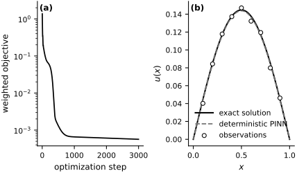
Fig. 58 Deterministic initialization. (a) Weighted inverse-PINN objective during optimization. (b) Exact state, deterministic PINN state, and observations. This optimizer output initializes NUTS; it is not the MAP estimate of the Bayesian model below.

Bayesian PINN Model

Let \(\mathbf{w}=(w_1,\ldots,w_{25})\) collect the network parameters and let \(\eta=\log\theta\). We assign the independent priors

\[ w_k \overset{\mathrm{iid}}{\sim} \mathcal{N}(0,1),\qquad \eta \sim \mathcal{N}(0,0.5^2),\qquad \theta=e^\eta. \]

The last transformation gives a lognormal prior for the positive conductivity. At the \(N_d=9\) sensor locations, the observation model is

\[ y_i \mid \mathbf{w} \sim \mathcal{N}(u_\mathbf{w}(x_i), \sigma_\mathrm{data}^2),\qquad \sigma_\mathrm{data}=0.003. \]

Define the residual

\[ r_\mathbf{w}(x;\theta)=-\theta u_\mathbf{w}''(x)-\sin(\pi x). \]

At the \(N_r=15\) collocation points, we use the pseudo-observation model

\[ 0 \mid \mathbf{w}, \theta \sim \mathcal{N}(r_\mathbf{w}(x_j;\theta), \sigma_\mathrm{PDE}^2),\qquad \sigma_\mathrm{PDE}=0.02. \]

Assuming conditional independence across sensors and collocation points, these factors and the priors define \(p(\mathbf{w},\eta\mid\mathbf{y},\mathbf{r}=\mathbf{0})\). The residual factor supplies the physics information at a finite set of points. Its scale \(\sigma_\mathrm{PDE}\) is a modeling tolerance, not measured process noise: decreasing it favors smaller residuals, and treating more collocation residuals as independent observations can also concentrate the posterior. The inference is conditional on this finite network, both noise scales, and the number and locations of collocation points.

sigma_pde = 0.02

def bpinn_model(x_obs, y_obs, x_phys):
    nn_params = numpyro.sample("nn_params", dist.Normal(0.0, 1.0).expand([n_nn_params]))
    log_theta = numpyro.sample("log_theta", dist.Normal(jnp.log(1.0), 0.5))
    theta = jnp.exp(log_theta)

    pred_obs = vmap(lambda x: pinn_solution(x, nn_params))(x_obs)
    pred_res = vmap(lambda x: pinn_residual(x, nn_params, theta))(x_phys)

    numpyro.sample("y", dist.Normal(pred_obs, noise_std).to_event(1), obs=y_obs)
    numpyro.sample("r", dist.Normal(pred_res, sigma_pde).to_event(1), obs=jnp.zeros_like(x_phys))

Posterior Sampling and Diagnostics

We run four sequential NUTS chains, using 1,000 warmup iterations and retaining 1,000 draws from each chain. Each transition differentiates through the network and its second spatial derivative at all collocation points, so this approach becomes expensive as the network and collocation set grow.

Neural-network parameterizations have symmetries, so individual weight coordinates can mix slowly even when the inferred conductivity and state are stable. We therefore report split-\(\widehat{R}\) and effective sample size for \(\theta\) and for the representative state value \(u(0.5)\), together with the number of divergent transitions. These observable summaries and the weight coordinates need not have the same mixing behavior.

init_values = {
    "nn_params": deterministic_params[:-1],
    "log_theta": deterministic_params[-1],
}

nuts = NUTS(
    bpinn_model,
    init_strategy=init_to_value(values=init_values),
    target_accept_prob=0.9,
)
mcmc = MCMC(
    nuts, num_warmup=1000, num_samples=1000, num_chains=4,
    chain_method="sequential", progress_bar=False,
)

key, mcmc_key = jr.split(key)
mcmc.run(mcmc_key, x_obs=x_obs, y_obs=y_obs, x_phys=x_phys)
posterior_by_chain = mcmc.get_samples(group_by_chain=True)
posterior = mcmc.get_samples()
divergences = int(mcmc.get_extra_fields()["diverging"].sum())

theta_by_chain = jnp.exp(posterior_by_chain["log_theta"])
theta_samples = jnp.exp(posterior["log_theta"])
u_mid_by_chain = vmap(
    vmap(lambda nn_params: pinn_solution(0.5, nn_params))
)(posterior_by_chain["nn_params"])
diagnostics = diagnostic_summary(
    {"theta": theta_by_chain, "u_mid": u_mid_by_chain}, group_by_chain=True
)
theta_diagnostics = diagnostics["theta"]
midpoint_diagnostics = diagnostics["u_mid"]

print("Chains: 4; warmup: 1,000 per chain; retained: 1,000 per chain")
print(f"Posterior mean conductivity: {theta_samples.mean():.4f}")
print(f"Posterior std conductivity:  {theta_samples.std():.4f}")
print(f"90% credible interval:       [{jnp.quantile(theta_samples, 0.05):.4f}, {jnp.quantile(theta_samples, 0.95):.4f}]")
print(f"theta R-hat / ESS:           {float(theta_diagnostics['r_hat']):.3f} / {float(theta_diagnostics['n_eff']):.0f}")
print(f"u(0.5) R-hat / ESS:          {float(midpoint_diagnostics['r_hat']):.3f} / {float(midpoint_diagnostics['n_eff']):.0f}")
print(f"Divergences:                 {divergences}")

Chains: 4; warmup: 1,000 per chain; retained: 1,000 per chain
Posterior mean conductivity: 0.7047
Posterior std conductivity:  0.0078
90% credible interval:       [0.6920, 0.7177]
theta R-hat / ESS:           1.008 / 250
u(0.5) R-hat / ESS:          1.004 / 405
Divergences:                 0

posterior_curves = vmap(
    lambda nn_params: vmap(lambda x: pinn_solution(x, nn_params))(xs_plot)
)(posterior["nn_params"])
curve_mean = posterior_curves.mean(axis=0)
curve_q05 = jnp.quantile(posterior_curves, 0.05, axis=0)
curve_q95 = jnp.quantile(posterior_curves, 0.95, axis=0)

theta_deterministic = jnp.exp(deterministic_params[-1])

fig, axes = new_figure("full_tall", nrows=2)

axes[0].fill_between(
    xs_plot, curve_q05, curve_q95, facecolor="0.65", edgecolor="none",
    linewidth=0.0, label="pointwise 90% interval"
)
axes[0].plot(
    xs_plot, curve_mean, color="black", linestyle="-",
    linewidth=0.7, label="posterior mean"
)
axes[0].plot(
    xs_plot, exact_solution(xs_plot), color="0.35", linestyle="--",
    linewidth=0.7, label="exact solution"
)
axes[0].plot(
    xs_plot, deterministic_pred, color="0.55", linestyle="-.",
    linewidth=0.7, label="deterministic PINN"
)
axes[0].scatter(
    x_obs, y_obs, s=20, facecolors="white", edgecolors="black",
    linewidths=0.8, zorder=3, label="observations"
)
axes[0].set(xlabel=r"$x$", ylabel=r"$u(x)$")
axes[0].legend(
    loc="lower center", bbox_to_anchor=(0.5, 1.02), ncol=3,
    borderaxespad=0.0, columnspacing=0.9, handlelength=2.4,
)

axes[1].hist(
    theta_samples, bins=24, density=True, facecolor="white",
    edgecolor="black", linewidth=0.7, hatch="///"
)
axes[1].axvline(
    true_theta, color="black", linestyle="--", linewidth=1.3,
    label="true conductivity"
)
axes[1].axvline(
    theta_deterministic, color="black", linestyle=":", linewidth=1.8,
    label="deterministic initializer"
)
axes[1].set(xlabel=r"$\theta$", ylabel="posterior density")
axes[1].legend(loc="lower center", bbox_to_anchor=(0.5, 1.02), ncol=2, borderaxespad=0.0)
label_panels(axes)
finalize_axes(axes)
plt.show()

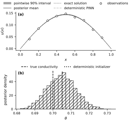
Fig. 59 Bayesian inverse-PINN posterior summaries. (a) Posterior mean of the latent state and the pointwise 90% credible interval, together with the exact and deterministic states and the observations. The interval excludes new measurement noise. (b) Marginal posterior density of the conductivity, with the true value and deterministic initializer shown for reference.

posterior_mean_curve = curve_mean
rel_l2_deterministic = (
    jnp.linalg.norm(deterministic_pred - exact_solution(xs_plot))
    / jnp.linalg.norm(exact_solution(xs_plot))
)
rel_l2_bayes = jnp.linalg.norm(posterior_mean_curve - exact_solution(xs_plot)) / jnp.linalg.norm(exact_solution(xs_plot))

print(f"Deterministic conductivity:  {float(theta_deterministic):.4f}")
print(f"Posterior mean conductivity: {float(theta_samples.mean()):.4f}")
print(f"Deterministic relative L2:   {float(rel_l2_deterministic):.4f}")
print(f"Posterior mean L2 error:     {float(rel_l2_bayes):.4f}")

Deterministic conductivity:  0.7052
Posterior mean conductivity: 0.7047
Deterministic relative L2:   0.0073
Posterior mean L2 error:     0.0070

The state and conductivity summaries are shown in Fig. 59. The deterministic initializer of this section (\(\theta\approx0.705\)) and the posterior mean (\(0.7047\)) are close because this manufactured inverse problem is well identified. For \(\theta>0\), the exact state \(u^\star(x;\theta)=\sin(\pi x)/(\theta\pi^2)\) is injective in \(\theta\) at every interior point where \(\sin(\pi x)\ne0\). With noisy data, the posterior is concentrated in this run, conditional on the selected priors and residual pseudo-likelihood.

The four-chain diagnostics above assess the identifiable conductivity and the representative state value \(u(0.5)\). Values of \(\widehat{R}\) near one, adequate effective sample sizes, and no divergent transitions provide evidence against obvious sampling failure for these summaries, but they do not establish that every neural-network weight coordinate has mixed.

The retained draws approximate the posterior distribution. The shaded region, which is barely wider than the plotted curves at this scale, is the pointwise interval between the 5th and 95th percentiles of the latent state \(u_\mathbf{w}(x)\); it is neither a simultaneous band nor a posterior-predictive interval for a new noisy observation. Its width reflects the model and sampling choices specified above.

Exercises

Rerun the companion notebook for each experiment. Report the posterior mean and 90% credible interval for \(\theta\), the \(\widehat{R}\) and effective sample size values, the number of divergences, and the relative \(L^2\) state error.

1. Create a fixed dense set of candidate sensor locations and one fixed noise realization. Compare nested subsets of these observations. How does the credible interval for \(\theta\) change as information is added?

2. Increase noise_std and regenerate the observations with the same random key. Compare the latent-state interval with a posterior-predictive interval that also includes new measurement noise. What happens at the two boundaries?

3. Decrease sigma_pde from 0.02 to 0.01. How do the posterior summaries and sampling diagnostics change? Explain why this changes the statistical model rather than only the numerical accuracy.

4. Replace the hidden layer with a wider one. Compare the state and conductivity summaries, and check whether the additional weight symmetries degrade the diagnostics.

5. Reduce the number of observations or increase their noise until the deterministic fit remains plausible but the conductivity posterior is broad. Explain what the point estimate alone conceals.