Show code cell source

Hide code cell source

import matplotlib.pyplot as plt
%matplotlib inline
import matplotlib_inline
matplotlib_inline.backend_inline.set_matplotlib_formats('svg')
import seaborn as sns

SINDy Example 2: Lorenz System

Here we replicate Example 2 in the appendix of Brunton et al. (2016). The Lorenz dynamics are:

\begin{align*} \dot{x} &= \sigma(y - x) \ \dot{y} &= x(\rho - z) - y \ \dot{z} &= xy - \beta z. \end{align*}

We take \(\sigma = 10\), \(\rho = 28\), and \(\beta = 8/3\).

import numpy as np
import scipy

sigma = 10.0
rho = 28.0
beta = 8.0 / 3.0
dt = 0.001
num_steps = int(100.0 / dt)
ts = np.linspace(0, 100, num_steps)
x0 = np.array([-8.0, 7.0, 27.0])

def vector_field(x, t):
    return (
        sigma * (x[1] - x[0]),
        x[0] * (rho - x[2]) - x[1],
        x[0] * x[1] - beta * x[2]
    )
xs = scipy.integrate.odeint(vector_field, x0, ts)

# Find the exact derivatives - no noise
from jax import vmap, jit
vf = jit(vmap(vector_field, in_axes=(0, 0)))
dxs = np.array(vf(xs, ts)).T

We use the sequential thresholded least-squares approach described by Brunton and Kutz (2019). We first fit least squares, set coefficients smaller than a threshold in magnitude to zero, and refit the surviving terms separately for each state derivative. Repeating these thresholding and refitting steps gives the sparse model. In the implementation below, alpha is the threshold:

def sparsify_dynamics(Phi, dxs, alpha, max_iter=100):
    """Solve the sparse regression problem to find the dynamics of the system.
    
    Args:
        Phi: The basis functions evaluated at each point in the state space.
        dxs: The time derivatives of the state space points.
        alpha: The sparsity parameter.
        max_iter: The maximum number of iterations to run the optimization.
    """
    thetas = np.linalg.lstsq(Phi, dxs, rcond=None)[0]
    d = dxs.shape[1]
    for _ in range(max_iter):
        smallinds = np.abs(thetas) < alpha
        thetas[smallinds] = 0
        for ind in range(d):
            biginds = smallinds[:, ind] == 0
            thetas[biginds, ind] = np.linalg.lstsq(Phi[:, biginds], dxs[:, ind], rcond=None)[0]
    return thetas

Solve the problem:

from sklearn.preprocessing import PolynomialFeatures

poly = PolynomialFeatures(degree=5)
Phi = poly.fit_transform(xs)

thetas = sparsify_dynamics(Phi, dxs, 0.025)

Let’s look at the coefficients:

for j in range(thetas.shape[1]):
    print(f"Dynamics of x_{j+1}:")
    print("-" * 20)
    for i, name in enumerate(poly.get_feature_names_out()):
        print(f"{name:10s} = {thetas[i][j]:.2f}") 

Show code cell output

Hide code cell output

Dynamics of x_1:
--------------------
1          = 0.00
x0         = -10.00
x1         = 10.00
x2         = 0.00
x0^2       = 0.00
x0 x1      = 0.00
x0 x2      = 0.00
x1^2       = 0.00
x1 x2      = 0.00
x2^2       = 0.00
x0^3       = 0.00
x0^2 x1    = 0.00
x0^2 x2    = 0.00
x0 x1^2    = 0.00
x0 x1 x2   = 0.00
x0 x2^2    = 0.00
x1^3       = 0.00
x1^2 x2    = 0.00
x1 x2^2    = 0.00
x2^3       = 0.00
x0^4       = 0.00
x0^3 x1    = 0.00
x0^3 x2    = 0.00
x0^2 x1^2  = 0.00
x0^2 x1 x2 = 0.00
x0^2 x2^2  = 0.00
x0 x1^3    = 0.00
x0 x1^2 x2 = 0.00
x0 x1 x2^2 = 0.00
x0 x2^3    = 0.00
x1^4       = 0.00
x1^3 x2    = 0.00
x1^2 x2^2  = 0.00
x1 x2^3    = 0.00
x2^4       = 0.00
x0^5       = 0.00
x0^4 x1    = 0.00
x0^4 x2    = 0.00
x0^3 x1^2  = 0.00
x0^3 x1 x2 = 0.00
x0^3 x2^2  = 0.00
x0^2 x1^3  = 0.00
x0^2 x1^2 x2 = 0.00
x0^2 x1 x2^2 = 0.00
x0^2 x2^3  = 0.00
x0 x1^4    = 0.00
x0 x1^3 x2 = 0.00
x0 x1^2 x2^2 = 0.00
x0 x1 x2^3 = 0.00
x0 x2^4    = 0.00
x1^5       = 0.00
x1^4 x2    = 0.00
x1^3 x2^2  = 0.00
x1^2 x2^3  = 0.00
x1 x2^4    = 0.00
x2^5       = 0.00
Dynamics of x_2:
--------------------
1          = 0.00
x0         = 28.00
x1         = -1.00
x2         = 0.00
x0^2       = 0.00
x0 x1      = 0.00
x0 x2      = -1.00
x1^2       = 0.00
x1 x2      = 0.00
x2^2       = 0.00
x0^3       = 0.00
x0^2 x1    = 0.00
x0^2 x2    = 0.00
x0 x1^2    = 0.00
x0 x1 x2   = 0.00
x0 x2^2    = 0.00
x1^3       = 0.00
x1^2 x2    = 0.00
x1 x2^2    = 0.00
x2^3       = 0.00
x0^4       = 0.00
x0^3 x1    = 0.00
x0^3 x2    = 0.00
x0^2 x1^2  = 0.00
x0^2 x1 x2 = 0.00
x0^2 x2^2  = 0.00
x0 x1^3    = 0.00
x0 x1^2 x2 = 0.00
x0 x1 x2^2 = 0.00
x0 x2^3    = 0.00
x1^4       = 0.00
x1^3 x2    = 0.00
x1^2 x2^2  = 0.00
x1 x2^3    = 0.00
x2^4       = 0.00
x0^5       = 0.00
x0^4 x1    = 0.00
x0^4 x2    = 0.00
x0^3 x1^2  = 0.00
x0^3 x1 x2 = 0.00
x0^3 x2^2  = 0.00
x0^2 x1^3  = 0.00
x0^2 x1^2 x2 = 0.00
x0^2 x1 x2^2 = 0.00
x0^2 x2^3  = 0.00
x0 x1^4    = 0.00
x0 x1^3 x2 = 0.00
x0 x1^2 x2^2 = 0.00
x0 x1 x2^3 = 0.00
x0 x2^4    = 0.00
x1^5       = 0.00
x1^4 x2    = 0.00
x1^3 x2^2  = 0.00
x1^2 x2^3  = 0.00
x1 x2^4    = 0.00
x2^5       = 0.00
Dynamics of x_3:
--------------------
1          = 0.00
x0         = 0.00
x1         = 0.00
x2         = -2.67
x0^2       = 0.00
x0 x1      = 1.00
x0 x2      = 0.00
x1^2       = 0.00
x1 x2      = 0.00
x2^2       = 0.00
x0^3       = 0.00
x0^2 x1    = 0.00
x0^2 x2    = 0.00
x0 x1^2    = 0.00
x0 x1 x2   = 0.00
x0 x2^2    = 0.00
x1^3       = 0.00
x1^2 x2    = 0.00
x1 x2^2    = 0.00
x2^3       = 0.00
x0^4       = 0.00
x0^3 x1    = 0.00
x0^3 x2    = 0.00
x0^2 x1^2  = 0.00
x0^2 x1 x2 = 0.00
x0^2 x2^2  = 0.00
x0 x1^3    = 0.00
x0 x1^2 x2 = 0.00
x0 x1 x2^2 = 0.00
x0 x2^3    = 0.00
x1^4       = 0.00
x1^3 x2    = 0.00
x1^2 x2^2  = 0.00
x1 x2^3    = 0.00
x2^4       = 0.00
x0^5       = 0.00
x0^4 x1    = 0.00
x0^4 x2    = 0.00
x0^3 x1^2  = 0.00
x0^3 x1 x2 = 0.00
x0^3 x2^2  = 0.00
x0^2 x1^3  = 0.00
x0^2 x1^2 x2 = 0.00
x0^2 x1 x2^2 = 0.00
x0^2 x2^3  = 0.00
x0 x1^4    = 0.00
x0 x1^3 x2 = 0.00
x0 x1^2 x2^2 = 0.00
x0 x1 x2^3 = 0.00
x0 x2^4    = 0.00
x1^5       = 0.00
x1^4 x2    = 0.00
x1^3 x2^2  = 0.00
x1^2 x2^3  = 0.00
x1 x2^4    = 0.00
x2^5       = 0.00

The identified dynamics reproduce the training data closely. We now make predictions with the identified model.

dt = 0.001
num_steps = int(250.0 / dt)
ts = np.linspace(0, 250, num_steps)

# Simulate with the original dynamics
xs = scipy.integrate.odeint(vector_field, x0, ts)

# Simulate with the learned dynamics
def f_learned(x, t, thetas, poly):
    phi = poly.fit_transform(x.reshape(1, -1)).flatten()
    dx = np.zeros(x.shape[0])
    for j in range(x.shape[0]):
        dx[j] = np.dot(thetas[:, j], phi)
    return dx

xs_learned = scipy.integrate.odeint(lambda x, t: f_learned(x, t, thetas, poly), x0, ts)

Compare visually the attractors:

fig = plt.figure(figsize=FIGURE_SIZES["full_standard"])
ax1 = fig.add_subplot(221, projection='3d')
steps = int(20/dt)
ax1.plot(xs[:steps, 0], xs[:steps, 1], xs[:steps, 2], lw=0.2)
ax1.set(xlabel='x', ylabel='y', zlabel='z', title='True Dynamics')
ax1.view_init(30, 120)

ax2 = fig.add_subplot(222, projection='3d')
ax2.plot(xs_learned[:steps, 0], xs_learned[:steps, 1], xs_learned[:steps, 2], lw=0.2)
ax2.set(xlabel='x', ylabel='y', zlabel='z', title='Learned Dynamics')
ax2.view_init(30, 120)

ax3 = fig.add_subplot(223, projection='3d')
ax3.plot(xs[:, 0], xs[:, 1], xs[:, 2], lw=0.2)
ax3.set(xlabel='x', ylabel='y', zlabel='z')
ax3.view_init(30, 120)

ax4 = fig.add_subplot(224, projection='3d')
ax4.plot(xs_learned[:, 0], xs_learned[:, 1], xs_learned[:, 2], lw=0.2)
ax4.set(xlabel='x', ylabel='y', zlabel='z')
ax4.view_init(30, 120);
fig.text(0.92, 0.5, "z", alpha=0)  # keeps the right-hand z labels inside the tight bounding box
plt.show()

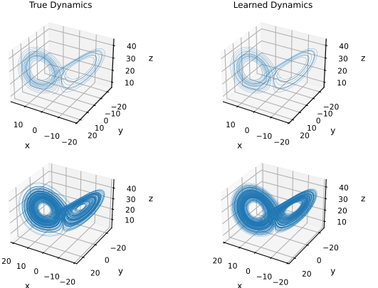
This replicates the first two columns of Figure 4 in the appendix of Brunton et al. (2016), without the color or noise. You see that the dynamics do not match perfectly (because the system is chaotic), but the attractors are very similar.

Let’s also plot the dynamo view:

fig = plt.figure(figsize=FIGURE_SIZES["full_standard"])
ax1 = fig.add_subplot(311)
steps = int(20/dt)
ax1.plot(ts[:steps], xs[:steps, 0], lw=1.0, label='True Dynamics')
ax1.plot(ts[:steps], xs_learned[:steps, 0], 'k--', lw=1.0, label='Learned Dynamics')
ax1.set(xlabel='Time', ylabel='x', title='True vs. Learned Dynamics')
finalize_axes(keep_box=False)

ax2 = fig.add_subplot(312)
ax2.plot(ts[:steps], xs[:steps, 1], lw=1.0, label='True Dynamics')
ax2.plot(ts[:steps], xs_learned[:steps, 1], 'k--', lw=1.0, label='Learned Dynamics')
ax2.set(xlabel='Time', ylabel='y')

ax3 = fig.add_subplot(313)
ax3.plot(ts[:steps], xs[:steps, 2], lw=1.0, label='True Dynamics')
ax3.plot(ts[:steps], xs_learned[:steps, 2], 'k--', lw=1.0, label='Learned Dynamics')
ax3.set(xlabel='Time', ylabel='z')
sns.despine(trim=True);

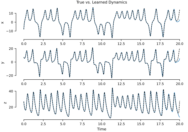
This reproduces Figure 5 in Brunton et al. (2016), without the noise.

Let’s repeat the same analysis, but this time we are going to add noise to the derivatives. The noise is zero mean, independent Gaussian with standard deviation \(\eta=10\).

# Noise level:
eta = 10.0

dxs_noisy = dxs + eta * np.random.randn(*dxs.shape)

# retrain
thetas_noisy = sparsify_dynamics(Phi, dxs_noisy, 0.025)

Repeat the plots above:

xs_learned = scipy.integrate.odeint(lambda x, t: f_learned(x, t, thetas_noisy, poly), x0, ts)

fig = plt.figure(figsize=FIGURE_SIZES["full_standard"])
ax1 = fig.add_subplot(221, projection='3d')
steps = int(20/dt)
ax1.plot(xs[:steps, 0], xs[:steps, 1], xs[:steps, 2], lw=0.2)
ax1.set(xlabel='x', ylabel='y', zlabel='z', title='True Dynamics')
ax1.view_init(30, 120)

ax2 = fig.add_subplot(222, projection='3d')
ax2.plot(xs_learned[:steps, 0], xs_learned[:steps, 1], xs_learned[:steps, 2], lw=0.2)
ax2.set(xlabel='x', ylabel='y', zlabel='z', title='Learned Dynamics')
ax2.view_init(30, 120)

ax3 = fig.add_subplot(223, projection='3d')
ax3.plot(xs[:, 0], xs[:, 1], xs[:, 2], lw=0.2)
ax3.set(xlabel='x', ylabel='y', zlabel='z')
ax3.view_init(30, 120)

ax4 = fig.add_subplot(224, projection='3d')
ax4.plot(xs_learned[:, 0], xs_learned[:, 1], xs_learned[:, 2], lw=0.2)
ax4.set(xlabel='x', ylabel='y', zlabel='z')
ax4.view_init(30, 120);
fig.text(0.92, 0.5, "z", alpha=0)  # keeps the right-hand z labels inside the tight bounding box

fig = plt.figure(figsize=FIGURE_SIZES["full_standard"])
ax1 = fig.add_subplot(311)
steps = int(20/dt)
ax1.plot(ts[:steps], xs[:steps, 0], lw=1.0, label='True Dynamics')
ax1.plot(ts[:steps], xs_learned[:steps, 0], 'k--', lw=1.0, label='Learned Dynamics')
ax1.set(xlabel='Time', ylabel='x', title='True vs. Learned Dynamics')
finalize_axes(keep_box=False)

ax2 = fig.add_subplot(312)
ax2.plot(ts[:steps], xs[:steps, 1], lw=1.0, label='True Dynamics')
ax2.plot(ts[:steps], xs_learned[:steps, 1], 'k--', lw=1.0, label='Learned Dynamics')
ax2.set(xlabel='Time', ylabel='y')

ax3 = fig.add_subplot(313)
ax3.plot(ts[:steps], xs[:steps, 2], lw=1.0, label='True Dynamics')
ax3.plot(ts[:steps], xs_learned[:steps, 2], 'k--', lw=1.0, label='Learned Dynamics')
ax3.set(xlabel='Time', ylabel='z')
sns.despine(trim=True);

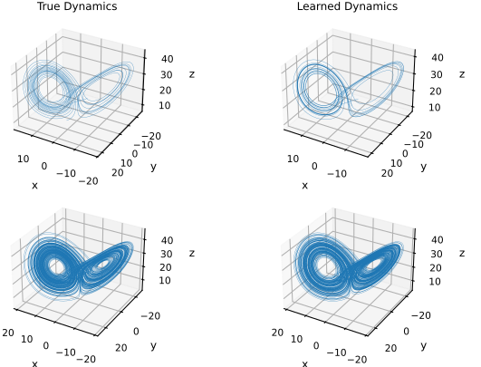
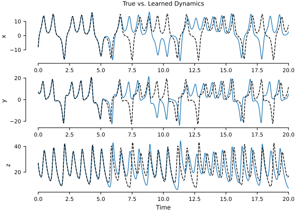
We see that the particular trajectories are not accurate after a while. The system is chaotic, so this is expected. Tiny errors will be magnified over time. The learned long-time geometry still resembles the reference attractor.