Example: The Catalysis Problem Using a Classical Approach

Example: The Catalysis Problem Using a Classical Approach#

This example uses the catalysis data reported by Tsilifis et al. (2016).

Consider the catalytic conversion of nitrate (\(\text{NO}_3^-\)) to nitrogen (\(\text{N}_2\)) and other by-products by electrochemical means. The mechanism that is followed is complex and not well understood. The experiments of Katsounaros et al. (2012) confirmed the production of nitrogen (\(\text{N}_2\)), ammonia (\(\text{NH}_3\)), and nitrous oxide (\(\text{N}_2\text{O}\)) as final products of the reaction, as well as the intermediate production of nitrite (\(\text{NO}_2^-\)).

The time is measured in minutes and the concentrations are measured in \(\text{mmol} \cdot \text{L}^{-1}\).

# Load the data in the units supplied by the source.
data_path = Path('../../data/catalysis.csv')
if not data_path.exists():
    url = 'https://raw.githubusercontent.com/PredictiveScienceLab/advanced-scientific-machine-learning/refs/heads/main/book/data/catalysis.csv'
    download(url)
    data_path = Path('catalysis.csv')
catalysis_data = pd.read_csv(data_path)
catalysis_data

	Time	NO3	NO2	N2	NH3	N2O
0	0	500.00	0.00	0.00	0.00	0.00
1	30	250.95	107.32	18.51	3.33	4.98
2	60	123.66	132.33	74.85	7.34	20.14
3	90	84.47	98.81	166.19	13.14	42.10
4	120	30.24	38.74	249.78	19.54	55.98
5	150	27.94	10.42	292.32	24.07	60.65
6	180	13.54	6.11	309.50	27.26	62.54

Let’s plot the data.

fig, ax = plt.subplots(figsize=FIGURE_SIZES["half_standard"])
time = catalysis_data['Time'].values
species_styles = ['-', '--', '-.', ':', (0, (5, 2)), (0, (3, 1, 1, 1))]
species_markers = ['o', 's', '^', 'D', 'v', 'P']
for i, col in enumerate([c for c in catalysis_data.columns if c != 'Time']):
    ax.plot(time, catalysis_data[col], color='black', linestyle=species_styles[i],
            marker=species_markers[i], markerfacecolor='white', label=col)
ax.legend(loc='upper center', bbox_to_anchor=(0.5, -0.20), ncol=3)
ax.set_xlabel('Time (min)')
ax.set_ylabel('Concentration (mmol L$^{-1}$)')
finalize_axes(keep_box=False)
plt.show()

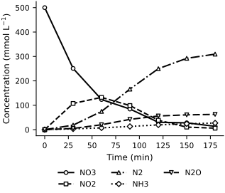
Observed concentrations of five chemical species versus time, distinguished by line style and marker.

The reported concentrations do not have a constant sum. We can inspect that sum using only the species columns. A molecular-concentration sum is not itself a mass balance: species contain different numbers of nitrogen atoms. We therefore use this calculation as a descriptive check, not as proof of a missing species.

catalysis_data[['NO3', 'NO2', 'N2', 'NH3', 'N2O']].sum(axis=1)

  500.00
  385.09
  358.32
  404.71
  394.28
  415.40
  418.95
dtype: float64

Katsounaros et al. (2012) proposed an unobserved intermediate X to explain the nitrogen-production dynamics. We use the simplified kinetic model and reported concentration convention reproduced by Tsilifis et al. (2016), without changing their data or rate equations.

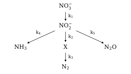
Nitrate forms nitrite at rate k1. Nitrite forms the unobserved intermediate X at rate k2, ammonia at rate k4, or nitrous oxide at rate k5. X forms nitrogen at rate k3.

The dynamical system associated with the reaction is:

\[\begin{split} \begin{aligned} \frac{d \left[\text{NO}_3^-\right]}{dt} &= -k_1\left[\text{NO}_3^-\right], \\ \frac{d\left[\text{NO}_2^-\right]}{dt} &= k_1\left[\text{NO}_3^-\right] - (k_2 + k_4 + k_5)[\text{NO}_2^-], \\ \frac{d \left[\text{X}\right]}{dt} &= k_2 \left[\text{NO}_2^-\right] - k_3 [\text{X}],\\ \frac{d \left[\text{N}_2\right]}{dt} &= k_3 \left[\text{X}\right], \\ \frac{d \left[\text{NH}_3\right]}{dt} &= k_4 \left[\text{NO}_2^-\right],\\ \frac{d \left[\text{N}_2\text{O}\right]}{dt} &= k_5 \left[\text{NO}_2^-\right], \end{aligned} \end{split}\]

where \([\cdot]\) denotes the concentration of a quantity, and \(k_i > 0\), \(i=1,\ldots,5\) are the kinetic rate constants.

Formulation of the Inverse Problem#

Step 1: Making our life easier by simplifying the notation#

Note that this is actually a linear system. To simplify our notation, let’s define:

\[\begin{split} \begin{array}{rcl} z_1 &:=& \left[\text{NO}_3^-\right],\\ z_2 &:=& \left[\text{NO}_2^-\right],\\ z_3 &:=& \left[\text{X}\right],\\ z_4 &:=& \left[\text{N}_2\right],\\ z_5 &:=& \left[\text{NH}_3\right],\\ z_6 &:=& \left[\text{N}_2\text{O}\right], \end{array} \end{split}\]

the vector:

\[ z = (z_1,z_2,z_3,z_4,z_5,z_6), \]

and the matrix:

\[\begin{split} A(k_1,\dots,k_5) = \left(\begin{array}{cccccc} -k_1 & 0 & 0 & 0 & 0 & 0\\ k_1 & -(k_2+k_4+k_5) & 0 & 0 & 0 & 0\\ 0 & k_2 & -k_3 & 0 & 0 & 0\\ 0 & 0 & k_3 & 0 & 0 & 0\\ 0 & k_4 & 0 & 0 & 0 & 0\\ 0 & k_5 & 0 & 0 & 0 & 0 \end{array}\right)\in\mathbb{R}^{6\times 6}. \end{split}\]

With these definitions, the dynamical system becomes:

\[ \dot{z} = A(k_1,\dots,k_5)z, \]

with initial conditions:

\[ z(0) = z_0 = (500, 0, 0, 0, 0, 0)\in\mathbb{R}^6, \]

read directly from the experimental data. We need a solver for this system. Let’s denote its solution at time \(t\) by:

\[ z(t;k_1,\dots,k_5). \]

Step 2: Scale the unknown parameters as well as possible#

Known physical constraints help restrict the plausible parameter values. We can enforce them through constrained optimization or through a suitable parameterization. Here, scaling the positive rate constants and taking logarithms gives unconstrained, dimensionless variables:

\(k_i\) has units of inverse time. It is appropriate to scale it with the total time, which is 180 minutes. So, let’s just multiply \(k_i\) with 180. This makes the resulting variable dimensionless:

\[ \hat{x}_i = 180k_i. \]

\(k_i\) is positive, therefore \(\hat{x}_i\) must be positive. So, let’s just work with the logarithm of \(\hat{x}_i\):

\[ x_i = \log \hat{x}_i = \log(180k_i). \]

define the parameter vector:

\[ x = (x_1,\dots,x_5)\in\mathcal{X} = \mathbb{R}^5. \]

From now on, we will write:

\[ A = A(x), \]

for the matrix of the dynamical system, and

\[ z = z(t;x), \]

for the solution at \(t\) given that the parameters are \(x\).

Step 3: Making the connection between our model and the experimental measurements#

Our experimental data include measurements of everything except \(z_3\) at six (6) time instants:

\[ t_j = 30j\;\text{minutes},\qquad j=1,\dots,6. \]

Now, let \(Y\in\mathbb{R}^{6\times 5}\) be the experimental measurements:

catalysis_data[1:]

	Time	NO3	NO2	N2	NH3	N2O
1	30	250.95	107.32	18.51	3.33	4.98
2	60	123.66	132.33	74.85	7.34	20.14
3	90	84.47	98.81	166.19	13.14	42.10
4	120	30.24	38.74	249.78	19.54	55.98
5	150	27.94	10.42	292.32	24.07	60.65
6	180	13.54	6.11	309.50	27.26	62.54

You can think of the measurements as a vector by flattening the matrix:

\[ y = \operatorname{vec}(Y)\in\mathbb{R}^{30}. \]

Note that \(\operatorname{vec}\) is the vectorization operator.

What is the connection between the solution of the dynamical system \(z(t;x)\) and the experimental data? It is as follows:

\[\begin{split} \begin{array}{ccc} z_1(30j;x) &\longrightarrow& Y_{j1},\\ z_2(30j;x) &\longrightarrow& Y_{j2},\\ z_4(30j;x) &\longrightarrow& Y_{j3},\\ z_5(30j;x) &\longrightarrow& Y_{j4},\\ z_6(30j;x) &\longrightarrow& Y_{j5}, \end{array} \end{split}\]

for \(j=1,\dots,6\).

We are now ready to define a function:

\[ f:\mathcal{X} \rightarrow \mathcal{Y}=\mathbb{R}^{30}_+, \]

as follows:

Define the matrix function:

\[ F:\mathcal{X} \rightarrow \mathbb{R}^{6\times 5}, \]

by:

\[\begin{split} \begin{array}{ccccc} F_{j1}(x) &=& z_1(30j;x)&\longrightarrow& Y_{j1},\\ F_{j2}(x) &=& z_2(30j;x) &\longrightarrow& Y_{j2},\\ F_{j3}(x) &=& z_4(30j;x) &\longrightarrow& Y_{j3},\\ F_{j4}(x) &=& z_5(30j;x) &\longrightarrow& Y_{j4},\\ F_{j5}(x) &=& z_6(30j;x) &\longrightarrow& Y_{j5}, \end{array} \end{split}\]

And flatten that function:

\[ f(x) = \operatorname{vec}(F(x))\in\mathbb{R}^{30}. \]

Now, we have made the connection with our theoretical formulation of inverse problems crystal clear.

Step 4: Programming our solver and the loss function#

First let’s define the system of ODEs.

# Define the linear system
def A(x):
    """
    Return the matrix of the dynamical system.
    """
    k = jnp.exp(x) / 180.0
    res = jnp.zeros((6, 6))
    res = res.at[0, 0].set(-k[0])
    res = res.at[1, 0].set(k[0])
    res = res.at[1, 1].set(-(k[1] + k[3] + k[4]))
    res = res.at[2, 1].set(k[1])
    res = res.at[2, 2].set(-k[2])
    res = res.at[3, 2].set(k[2])
    res = res.at[4, 1].set(k[3])
    res = res.at[5, 1].set(k[4])
    return res

def dynamic_sys(t, z, x):
    return jnp.dot(A(x), z)

Now, let’s use diffrax for our ODE solver. We have to extract the experiment times, even though our ODE does not depend on it, the solver needs to know how long to solve the ODE for and where to save the solution.

# Experimental times
t_exp = jnp.array(catalysis_data.loc[catalysis_data['Time'] > 0, 'Time'].values)
t0 = 0.0
t1 = t_exp[-1]

# Solve the ODE using Diffrax
def solve_catalysis(t, x, z0):

    sol = diffeqsolve(
        ODETerm(dynamic_sys),
        Tsit5(),
        t0=t0,
        t1=t1,
        dt0=0.1,
        y0=z0,
        args=x,
        saveat=SaveAt(ts=t),
        max_steps=100_000,
    )
    return sol.ys

We can solve this ODE and find the model parameters by minimizing a loss function. Here we extract the result of the solver for the concentrations that we measure and compare it to the experimental data.

# Define the loss function to minimize
def loss(x, z, y, t):

    # Compute the solution
    res = solve_catalysis(t, x, z)

    # Extract the concentration of the species of interest
    flat_res = jnp.hstack([res[:, :2], res[:, 3:]]).flatten()

    # Scaled for numerical stability
    loss_val = 0.5 * jnp.sum((flat_res / 500. - y / 500.) ** 2) 

    return loss_val

Via this loss function, we can use Adam to do gradient descent and find the model parameters that best fit the data.

# Initial guess for x
key = jr.PRNGKey(0)
x0 = jr.normal(key, shape=(5,))  

# Initial conditions
z0 = jnp.array([500., 0., 0., 0., 0., 0.0])

# Extract the experimental data
Y = catalysis_data.loc[catalysis_data['Time'] > 0, ['NO3', 'NO2', 'N2', 'NH3', 'N2O']].values
y = Y.flatten()

# Set up the optimizer
optimizer = optax.adam(learning_rate=1e-1)
opt_state = optimizer.init(x0)

x = x0  # Initialize x

# Use as many iterations as needed
num_iterations = 100
loss_evol = []

# Optimization loop
for i in range(num_iterations):

    # Compute the gradient of the loss function
    grad_fn = jit(grad(loss))

    grads = grad_fn(x, z0, y, t_exp)

    # Update the optimizer state
    updates, opt_state = optimizer.update(grads, opt_state)

    # Update the parameters
    x = optax.apply_updates(x, updates)

    value = loss(x, z0, y, t_exp)
    loss_evol.append(value)
    
    # Print the loss every 100 iterations
    if i % 10 == 0:
        print(f"Iteration {i}, loss: {value}")

Iteration 0, loss: 1.0947077944734844

Iteration 10, loss: 0.2773287530113111

Iteration 20, loss: 0.07561202249882777

Iteration 30, loss: 0.06467950730878569

Iteration 40, loss: 0.02874868527847827

Iteration 50, loss: 0.025166677247283394

Iteration 60, loss: 0.014660491022276451

Iteration 70, loss: 0.008768475795593752

Iteration 80, loss: 0.007619054958603772

Iteration 90, loss: 0.007624082179164428

Let’s see how the minimization went.

fig, ax = plt.subplots(figsize=FIGURE_SIZES["half_standard"])
ax.plot(loss_evol)
ax.set_xlabel('Iteration')
ax.set_ylabel('Loss')
finalize_axes(keep_box=False)
plt.show()

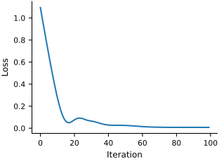
Optimization loss decreases over iterations toward a stable minimum.

Great, it looks like it has converged. Let’s plot the results of the model against our experimental data to see how well we did.

x_est = x
t_exp = jnp.array(catalysis_data['Time'].values)

# Generate predictions using the estimated parameters
t_plot = jnp.linspace(0.0, 180.0, 100)
Yp = solve_catalysis(t_plot, x_est, z0)

# Plotting
fig, ax = plt.subplots(figsize=FIGURE_SIZES["half_standard"])

# Define labels and colors
labels = ['NO3-', 'NO2-', 'N2', 'NH3', 'N2O', 'X']
data_cols = ['NO3', 'NO2', 'N2', 'NH3', 'N2O']
model_cols = [0, 1, 3, 4, 5, 2]
species_styles = ['-', '--', '-.', ':', (0, (5, 2)), (0, (3, 1, 1, 1))]
species_markers = ['o', 's', '^', 'D', 'v', 'P']

# Plot experimental data
for i, col in enumerate(data_cols):
    ax.plot(t_exp, catalysis_data[col], linestyle='none', color='black',
            marker=species_markers[i], markerfacecolor='white',
            label=f'Data {labels[i]}')

# Plot model predictions
for i, col in enumerate(model_cols):
    ax.plot(t_plot, Yp[:, col], color='black', linestyle=species_styles[i],
            label=f'Model {labels[i]}')

ax.set_xlabel('Time (min)')
ax.set_ylabel(r'Concentration (mmol L$^{-1}$)')
ax.legend(loc='upper center', bbox_to_anchor=(0.5, -0.20), ncol=2)
finalize_axes(keep_box=False)
plt.show()

print("Estimated parameters x:", x_est)

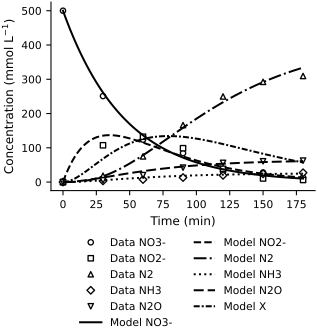
Observed and fitted concentrations of six chemical species versus time; markers denote data and styled curves denote the model.

Estimated parameters x: [ 1.35978812  1.704498    1.29209594 -1.06225672 -0.15488091]

Exercises#

Are you satisfied with the above model calibration?
Rerun the code with a different seed. Does the algorithm always work? Do you find exactly the same \(x\)?
Start from an initial \(x\) that is very far away from the zero. Like all 10’s. What do you find?
What is the average number of function evaluations that you need? Can this method be easily applied to expensive models?

Shortcomings of the Classical Approach#

There are several shortcomings of the classical approach to model calibration that the Bayesian formulation addresses. Here we briefly mention some:

The problems are ill-posed. Solutions may not exist, or more than one solution may exist.
No apparent way to quantify uncertainties.
No systematic way to account for prior knowledge.