
Hierarchical Model Structure#
A hierarchy becomes precise once we specify the conditional distribution at each layer of the data-generating process. Population modeling provides a concrete example: related experiments have local parameters that vary around a shared distribution. The same structure also applies when the shared quantities represent common physical conditions, calibration variables, or other features that connect several data-producing units.
The basic pattern#
Consider \(N\) related data-producing units indexed by \(i=1,\ldots,N\). Let \(\phi\) denote global unknowns shared by all units, \(\theta_i\) the local unknowns for unit \(i\), and \(y_i\) the data observed from that unit. A simple hierarchical model generates these quantities in the order
The resulting joint density factorizes as
Here, \(p(\phi)\) is a hyperprior: a prior on the parameters that govern the local distributions.
A probabilistic graphical model (PGM) displays the same factorization. Each circle is a random variable, and shading marks an observed variable. An arrow points to a variable whose conditional distribution depends directly on its parent. These arrows encode the probabilistic factorization; they do not by themselves assert a physical causal relationship. A rectangle, called a plate, repeats the enclosed structure over its index. For a broader introduction to probabilistic graphical models and plate notation, see Bishop (2006), Chapter 8.
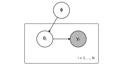
Fig. 24 The basic hierarchical pattern. The local variable \(\theta_i\) and observation \(y_i\) are repeated for \(i=1,\ldots,N\), while \(\phi\) lies outside the plate because it is shared by all units.#
Conditional on \(\phi\), the local variables \(\theta_1,\ldots,\theta_N\) are independent under this factorization. After \(\phi\) is integrated out, they are generally dependent because they share the same uncertain global quantity. Likewise, observations from different units are conditionally independent once their local variables are known, but they remain statistically connected through the hierarchy.
Partial pooling#
In a population model, the hierarchy produces partial pooling (Gelman et al., 2013). A unit with abundant data can support a local parameter far from the population mean, whereas a unit with limited data is informed more strongly by the shared population distribution. If the units are similar, the posterior learns a small between-unit spread; if they are heterogeneous, it can learn a larger spread.
Partial pooling lies between two limiting models. No pooling fits each unit independently and does not share information. Complete pooling forces every unit to have the same parameter. Partial pooling instead learns how much information should be shared. This is useful for repeated experiments involving different specimens, subjects, sensors, trajectories, or manufactured components.
Hyperpriors#
The global quantities are unknown and therefore require priors of their own. For a scalar local parameter, for example, one may write
where \(\mu\) is the population mean and \(\tau>0\) is the population standard deviation. Priors on \(\mu\) and \(\tau\) are hyperpriors. The prior on \(\tau\) is especially consequential: small values produce stronger pooling, whereas large values permit greater between-unit variation. When the data constrain \(\tau\) only weakly, the posterior can have narrow, strongly coupled regions. The following examples show both the inferential benefits of this structure and the computational consequences of its geometry.