import matplotlib.pyplot as plt
%matplotlib inline
import matplotlib_inline
matplotlib_inline.backend_inline.set_matplotlib_formats('svg')
import seaborn as sns
Connection Between SVD and Principal Component Analysis#
PCA is a linear dimensionality-reduction technique. We typically use PCA in supervised or unsupervised learning to reduce the number of features in the dataset. The main idea behind PCA is to find a new set of features that are uncorrelated and ordered by the amount of variance they explain.
Let \(\mathbf{X}\) be an \(n \times m\) matrix, where \(n\) is the number of samples and \(m\) is the number of features. We will use \(\mathbf{x}_i\) to denote the \(i\)-th row of \(\mathbf{X}\). So, write:
where:
When we do PCA, we always want to center the data. To this end, we calculate the empirical mean of the data:
and we make the centered data matrix:
Now take an arbitrary unit vector \(\mathbf{v}\).
array([<Axes: >], dtype=object)
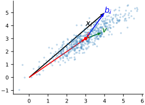
Consider the projection of the centered sample \(\mathbf{b}_i=\mathbf{x}_i-\bar{\mathbf{x}}\) (the \(i\)-th row of \(\mathbf{B}\)) on \(\mathbf{v}\). It is:
What is the empirical mean of the projections?
because \(\mathbf{b}_i\) is centered.
What is the variance of the projections?
where \(\mathbf{C}\) is the covariance matrix of the centered data:
PCA finds \(\mathbf{v}\) by solving the following problem:
subject to the constraint that \(\mathbf{v}\) is a unit vector.
Using the method of Lagrange multipliers, we can show that the solution to this problem is the eigenvector of \(\mathbf{C}\) with the largest eigenvalue.
In a similar way, we can find the second principal direction, \(\mathbf{v}_2\). And so on. We always get a sequence of orthogonal unit vectors, \(\mathbf{v}_1, \mathbf{v}_2, \ldots, \mathbf{v}_m\), corresponding to the eigenvalues of \(\mathbf{C}\) in decreasing order.
And now, here is the connection between PCA and SVD. Do the SVD of the centered matrix \(\mathbf{B}\):
Here \(\mathbf{\Sigma}\) is \(n\times m\), so \(\mathbf{\Sigma}^T\mathbf{\Sigma}\) is an \(m\times m\) diagonal matrix. If \(m>n\), its last \(m-n\) entries are zero. Form the covariance:
So, we get that the SVD diagonalizes the covariance matrix. We can read off the eigenvalues and eigenvectors. The \(j\)-th column of \(\mathbf{V}\) is the \(j\)-th principal direction. The \(j\)-th singular value squared and divided by \(n\) is the variance in the \(j\)-th principal direction.
The total variance of the data is:
The projection coefficients are known as the principal components. They are:
Example: PCA on the MNIST dataset#
We use the MNIST dataset (LeCun et al., n.d.) to illustrate PCA. The notebook loads OpenML dataset 554 (mnist_784, version 1).
from sklearn.datasets import fetch_openml
mnist = fetch_openml('mnist_784', version=1)
Let’s do the steps described above:
import numpy as np
# 1. Extract the relevant data
X = mnist.data
# 2. Find the empirical mean
x_bar = np.mean(X, axis=0)
# 3. Center the data
B = X - x_bar
# 4. Do the SVD
U, S, Vt = np.linalg.svd(B, full_matrices=False)
# 5. Project the data
Z = U @ np.diag(S)
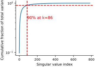
Let’s look at the explained variance:
array([<Axes: xlabel='Singular value index', ylabel='Cumulative fraction of total variance'>],
      dtype=object)
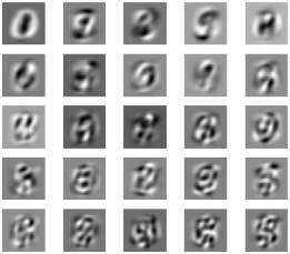
Let’s look at the first 10 principal directions:
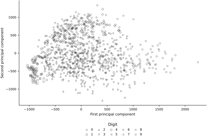
We fit PCA to all 70,000 images and display a fixed random subset of 100 images per digit. Marker shapes identify the digits; subsampling keeps the overlapping groups visible.
y = np.asarray(mnist.target, dtype=int)
display_rng = np.random.default_rng(697)
markers = ["o", "s", "^", "v", "D", "<", ">", "p", "h", "8"]
fig, ax = plt.subplots(
    figsize=FIGURE_SIZES["full_standard"], constrained_layout=True
)
for digit, marker in enumerate(markers):
    mask = display_rng.choice(np.flatnonzero(y == digit), size=100, replace=False)
    ax.scatter(
        Z[mask, 0],
        Z[mask, 1],
        label=str(digit),
        marker=marker,
        s=16,
        facecolors="none",
        edgecolors="black",
        linewidths=0.55,
        alpha=0.65,
    )
ax.legend(
    loc="upper center", bbox_to_anchor=(0.5, -0.14),
    ncol=5, title="Digit", handletextpad=0.35, columnspacing=0.9,
)
ax.set(xlabel="First principal component", ylabel="Second principal component")
finalize_axes(keep_box=False)
array([<Axes: xlabel='First principal component', ylabel='Second principal component'>],
      dtype=object)