Show code cell source

Hide code cell source

import numpy as np
import matplotlib.pyplot as plt
%matplotlib inline
import matplotlib_inline
matplotlib_inline.backend_inline.set_matplotlib_formats('svg')
import seaborn as sns

Numerical Differentiation

Take a function \(f:\mathbb{R} \rightarrow \mathbb{R}\) and a point \(x_0 \in \mathbb{R}\). The derivative of \(f\) at \(x_0\) is defined as

\[ f'(x_0) = \lim_{h \rightarrow 0} \frac{f(x_0 + h) - f(x_0)}{h}. \]

Numerical differentiation uses a finite value of \(h\) to approximate the derivative. The simplest method is to use a forward difference:

\[ f'(x_0) \approx \frac{f(x_0 + h) - f(x_0)}{h}. \]

Let’s write code that implements this approximation. We will use this as an excuse to revisit higher-order functions in Python. These are functions that take other functions as arguments or return functions as results. The programming paradigm that uses higher-order functions is called functional programming.

Here it is:

def make_numerical_grad(f, h=1e-4):
    """Return a function that evaluates the derivative of f at any point."""
    def grad(x):
        return (f(x + h) - f(x)) / h
    return grad

Here is how to use this:

f = lambda x: x**3
df = make_numerical_grad(f)
type(df)

function

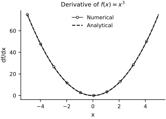
Let’s plot it:

fig, ax = plt.subplots(
    figsize=FIGURE_SIZES["half_standard"], constrained_layout=True
)
x = np.linspace(-5, 5, 100)
ax.plot(
    x, df(x), color="0.35", linewidth=1.2, marker="o",
    markerfacecolor="white", markeredgecolor="0.20",
    markersize=3.5, markevery=10, label="Numerical",
)
ax.plot(
    x, 3*x**2, color="0.0", linestyle="--", linewidth=1.3,
    label="Analytical",
)
ax.legend(loc='best', frameon=False)
ax.set(xlabel='x', ylabel='df/dx', title='Derivative of $f(x)=x^3$')
finalize_axes(keep_box=False)
plt.show()

Let’s now move to multivariate functions. Take a function \(f:\mathbb{R}^n \rightarrow \mathbb{R}\) and a point \(\mathbf{x}_0 \in \mathbb{R}^n\). The derivative of \(f\) at \(\mathbf{x}_0\) is defined as the column vector:

\[ \nabla f(\mathbf{x}_0) = \left[ \partial_1 f(\mathbf{x}_0), \ldots, \partial_n f(\mathbf{x}_0) \right]^{\mathsf T} \]

where

\[ \partial_i f(\mathbf{x}_0) = \lim_{h \rightarrow 0} \frac{f(\mathbf{x}_0 + h \mathbf{e}_i) - f(\mathbf{x}_0)}{h} \]

Notice that our notation is slightly different from the classical notation used in math textbooks. We write \(\partial_i f\) instead of \(\frac{\partial f}{\partial x_i}\). When we write \(\partial_i f\) we mean the partial derivative of the function \(f\) with respect to the \(i\)-th argument. This notation saves us quite a bit of typing.

Let’s write a function that computes this derivative using numerical differentiation on NumPy arrays (np is numpy).

def make_numerical_grad_mv(f, h=1e-4):
    """Return a function that evaluates the derivative of a multivariate f at any point."""
    def grad(x):
        grad = np.zeros_like(x)
        fx =  f(x)
        for i in range(len(x)):
            x_plus_h = x.copy()
            x_plus_h[i] += h
            grad[i] = (f(x_plus_h) - fx) / h
        return grad
    return grad

Let’s test it with:

\[ f(x) = x_1^3 + x_2^2 + x_3^4 \]

which has a gradient:

\[ \nabla f(\mathbf{x}) = \left[ 3 x_1^2, 2 x_2, 4 x_3^3 \right]^T. \]

def f(x):
    return x[0] ** 3 + x[1] ** 2 + x[2] ** 4

gf = make_numerical_grad_mv(f)

x = np.array([1.0, 1.0, 1.0])

gf(x)

array([3.00030001, 2.0001    , 4.00060004])

The approximation agrees closely with the exact gradient. Numerical differentiation nevertheless has two limitations: accuracy and computational cost.

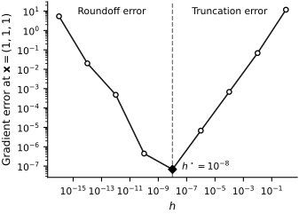
Let’s talk about accuracy first. The accuracy of numerical differentiation depends on the value of \(h\). A very small \(h\) amplifies cancellation and roundoff in the difference, while a large \(h\) causes truncation error. There is a trade-off between these two sources of error. The optimal value of \(h\) depends on the function \(f\) and the point \(x_0\). Choosing \(h\) therefore requires information about derivative and rounding-error scales. Let’s demonstrate this with an example.

hs = np.logspace(-16, 0, 9)
errors = []
for h in hs:
    gf = make_numerical_grad_mv(f, h=h)
    errors.append(np.linalg.norm(gf(x) - np.array([3, 2, 4])))

fig, ax = plt.subplots(
    figsize=FIGURE_SIZES["half_standard"], constrained_layout=True
)
ax.plot(
    hs, errors, color="0.10", linewidth=1.2, marker="o",
    markerfacecolor="white", markeredgecolor="black", markersize=4,
)
optimal_h = hs[np.argmin(errors)]
ax.axvline(optimal_h, linestyle="--", color="0.45", linewidth=1.0)
ax.scatter(
    optimal_h, np.min(errors), marker="D", s=24, color="black",
    zorder=3,
)
ax.annotate(
    rf"$h^\star=10^{{{int(round(np.log10(optimal_h)))}}}$",
    xy=(optimal_h, np.min(errors)), xytext=(8, -2),
    textcoords="offset points", ha="left", va="bottom",
    fontsize=8,
)
ax.text(
    0.12, 0.97, "Roundoff error", transform=ax.transAxes,
    ha="left", va="top", fontsize=8,
)
ax.text(
    0.88, 0.97, "Truncation error", transform=ax.transAxes,
    ha="right", va="top", fontsize=8,
)
ax.set(
    xlabel="$h$", ylabel=r"Gradient error at $\mathbf{x}=(1,1,1)$",
    xscale="log", yscale="log",
)
finalize_axes(keep_box=False)
plt.show()

The second problem is speed. To evaluate the gradient we need to evaluate the function \(n+1\) times. This cost grows with the number of model parameters. Imagine having a neural network with a million parameters and that you want to find the gradient of the loss function with respect to all the parameters. You would need to evaluate the loss function a million times plus one for each iteration of gradient descent. That cost is prohibitive for large models.